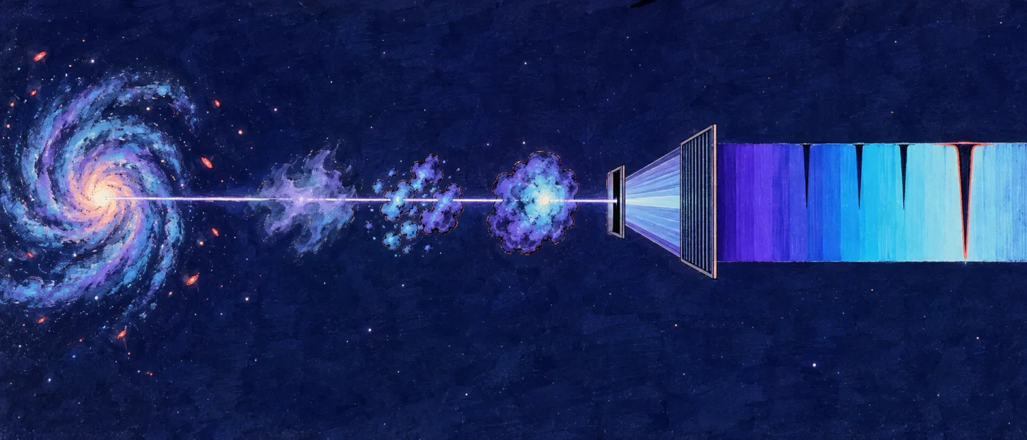
Eleven absorber updates: a 0.95 Å completeness floor, a galaxy–forest peak 10 cMpc inside the measured one, and a U-Net whose every confident error sits near a damped absorber
Eleven papers show what each measurement's own sample size and detection threshold decide before a simulation can be measured against it, from a sodium survey that can claim only half its absorbers above 0.95 Å to a mock galaxy–forest correlation whose peak sits 10 cMpc inside the observed one.

Three of this week's eleven items set a synthetic observable against a measured counterpart of it. One sets a measured distribution against a hydrodynamical run. Two generate their observable from a simulation and stop there. Five report measurements with no simulation anywhere in the comparison. 1234567891011
Five of the eleven put their decisive number on the size or the threshold of their own sample rather than on the physics. A blind search for sodium doublets along 214,035 DESI quasar sightlines finds 3,636 of them but can claim only half of the absorbers above a rest equivalent width of 0.95 Å, so the absorber statistics rest on the 1,336 above that floor. A neural network asked to find metal lines in survey-like mock spectra reaches ninety per cent on completeness, purity and F1 only at a line signal-to-noise of four, and all seventeen of its mistakes above a line signal-to-noise of five sit beside a damped absorber. A mock survey built to the ASPIRE specification returns a Kolmogorov–Smirnov p-value of 0.441 between sightlines biased towards galaxies and random ones, and the paper works out that separating the two takes roughly ten times the survey. A forward model of the same galaxy-to-forest statistic in mock JWST catalogues puts its own correlation peak 10 cMpc inside the measured one and calls the offset smaller than the scatter among its realisations. And a 21-cm survey that finds five absorbers reports three per cent once its own optical-depth cut is applied, against five per cent raw.
The measurements behind them start at low redshift. Sodium absorbers become 3.4 times more common between redshift 0.25 and redshift 0.03; circumgalactic dust around low-redshift galaxies scales as the halo mass to 0.69; damped absorbers sit closer to their galaxies the more metal-rich they are; the cosmic-noon circumgalactic medium is already as enriched as today's; and the Large Magellanic Cloud's wind thins out between 125 and 200 kilometres per second of outflow speed, in gas that is not all the Cloud's.
The order below follows that grouping: the low-redshift measurements first, the two simulation-to-observation comparisons next, then the galaxy–absorber, benchmark and local-sightline items, and the three method papers last.
Quick look
The class in each row reads as follows: (a) a synthetic observable set against real data, meaning a simulation's own mock product is compared with a measured counterpart of that same observable; (b) a benchmark at the level of physical quantities, in which a model or a measurement is set against hydrodynamical runs and the mock spectra are left aside; (c) a synthetic-only result, with no observed counterpart of the synthetic observable in the comparison; (d) an observational anchor, a real measurement with no simulation in the comparison.
| Work | Class and redshift | Comparison level | Result to screen on | Code and data |
|---|---|---|---|---|
| Anand & Muzahid, arXiv:2609.26794 | (d) observational anchor; 0.01 ≲ z ≲ 0.27 | 3,636 Na Iλλ5891,5897 doublets in 214,035 DESI DR1 quasar sightlines, with an injection–recovery selection function | dN/dX falls by 3.4 ± 0.34 from z ≈ 0.03 to z ≈ 0.25 on the 1,336 absorbers above a 0.95 Å completeness floor; catalogue purity 77% 1 | Three public fitting packages named; the pinned qsoabsfind version and the printed Zenodo DOI do not resolve 12 |
| Genc et al., arXiv:2609.34615 | (d) observational anchor; z_B < 0.42 | KiDS-DR5 galaxy–galaxy lensing plus a nine-band magnitude shift in five stellar-mass bins, 3,254,554 lenses | Halo mass log M_c from 11.66 to 12.63, dust mass log M_d1 from 7.53 to 8.02; M_dust ∝ M_halo^(0.69 ± 0.19) 2 | No repository, no data DOI and no URL printed anywhere 13 |
| Deka et al., A&A 713, A319 | (d) observational anchor; 0.29 < z < 0.47 | MALS MeerKAT 21-cm absorption in 99 radio-loud AGN with S_1.4GHz > 4 mJy, against sensitivity-matched WSRT and VLA samples | Five detections (four LERGs, one HERG) and a rate of 3 (+3/−2) % at a 3σ ∫τ dv cut of 10.0 km s⁻¹ 3 | GELATO public under GPL-3.0; the classified catalogue is electronic-only and no data DOI is printed 1415 |
| Anderson et al., arXiv:2609.26483 | (a) synthetic observable against real data; 5.4 < z < 6.1 | Mock Lyα-forest τ_eff near mock [O III] emitters in one Sherwood-Relics run, against the ASPIRE τ_eff distributions | One mock ASPIRE survey gives a median KS statistic of 0.20 and p = 0.441; separating biased from random sightlines needs about ten times the ASPIRE sightline length 4 | No repository and no data DOI printed; Sherwood-Relics data by email request 16 |
| Conaboy et al., OJAp 9 | (a) synthetic observable against real data; z ≈ 6 | Mock JWST [O III] catalogues from Sherwood-Relics against the measured galaxy–transmission cross-correlation at three redshifts | Mock δ_F peaks at r ≈ 20 cMpc against a measured r ≈ 30 cMpc, with 0.3 ≲ Σ/⟨Σ⟩ ≲ 1.6 of realisation scatter, which the paper reads as no tension 5 | No repository and no data DOI; the authors' code on request 17 |
| Oyarzún et al., arXiv:2609.25221 | (d) observational anchor; z ≈ 3–5 | 36 DLAs along 17 sightlines with Keck/KCWI integral-field Lyα imaging, out to b ≲ 120 kpc | 7 DLA Lyα emitters found; on 11 emitters with MAGG, impact parameter falls below 50 kpc as [M/H] reaches −1, at 1.8σ from a Monte Carlo 6 | No repository; the arXiv related DOI does not resolve; HST imaging DOI printed 18 |
| Deepak et al., arXiv:2609.26785 | (b) physical-level benchmark; 1 ≤ z ≤ 2.2 | 105 H I-selected absorbers with HST UV and Keck/VLT optical spectra, against published EAGLE metallicity distributions | Median [X/H] = −1.19, statistically indistinguishable from −1.18 at z < 1; EAGLE matches z = 1 better than z = 2 despite ⟨z⟩ = 1.81 7 | pyigm and rbcodes public; machine-readable tables promised with no address 1920 |
| Poudel et al., arXiv:2609.32137 | (d) observational anchor; z = 0 | 170 ULLYSES OB stars behind the LMC, with Voigt-profile fits and Cloudy modelling of 13 sightlines | Mean Si II column reaches its minimum between v_LMCSR ≈ −200 and −125 km s⁻¹; the fast gas mixes LMC wind, Magellanic and Milky Way material 8 | Spectra public on GitHub with no licence and no tagged release 21 |
| Mangola et al., arXiv:2609.28072 | (c) synthetic-only; quasar rest frame 1230–3095 Å | A 1D U-Net on 50,000 WEAVE-like mock spectra, ~35,000 for training, with a simulated continuum-fitting step | Completeness, purity and F1 all reach 90% at a line signal-to-noise of 3.80; 17 false positives above 5 all sit near damped absorbers 9 | No code repository; trained models on Zenodo under CC BY 4.0 22 |
| Karam et al., arXiv:2609.32582 | (c) synthetic-only; z = 0 | AstroCLIP embeddings of 1,704 mock Chandra images from TNG300 and TNG-Cluster, predicting central cooling time | RMSE 0.24 and 0.23 dex in-simulation; trained on one simulation and tested on the other, 0.503 dex against 0.729 for a fine-tuned CNN 10 | No repository of its own; no data DOI; the Data Availability section is MNRAS template text 23 |
| Abghari et al., arXiv:2609.25548 | (a) synthetic observable against real data; full-sky projection, no redshift printed | Planck 2015 MILCA and NILC tSZ maps against Websky, Sehgal et al., Magneticum and eleven HalfDome realisations | The excess second-order scattering coefficient of MILCA exceeds every simulation at every scale; no printed statistic accompanies the claim 11 | HAWCS public under MIT, newest commit 18 September 2026, no tags and not on PyPI 24 |
Every entry below carries the same five fields: sample and observable, method and result, real-data stage and caveat, code and data, and why open it.
1. Anand and Muzahid: sodium absorbers grow by 3.4 times towards the present, on the 1,336 that clear the completeness cut
Abhijeet Anand and Sowgat Muzahid posted The First Blind Survey of Intervening Na I Absorbers: Incidence and Cosmic Evolution with DESI on 22 September at 12:59 p.m. Central Time, and the astro-ph.GA listing carried it on 23 September. 1
Sample and observable. The search runs over 214,035 quasar sightlines from DESI Data Release 1, each with a median per-pixel signal-to-noise of at least 7 inside the sodium window. It returns 3,636 Na I λλ5891,5897 doublets between z_abs = 0.01 and z_abs = 0.27, at a mean redshift of 0.13, which puts every detection at low redshift and none of them beyond a lookback time of a few billion years. The absorbers are found by matched filtering rather than by eye, and the doublet alone carries the identification, since the two lines are separated by a fixed 6 Å in the rest frame. 25
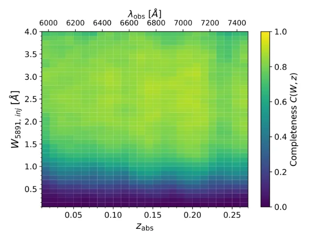
Method and result. The selection function is measured rather than argued. Roughly 650,000 absorbers were injected into the real spectra, at least three per quasar, with rest equivalent widths drawn uniformly from 0.1 to 4.0 Å, doublet ratios from 1 to 2 and velocity dispersions around 30 to 130 km s⁻¹, and then recovered by the same pipeline. Completeness reaches 50% at W_5891 = 0.95 Å, climbs to about 85% between 1.9 and 2.0 Å, stays roughly flat out to 3.5 Å and declines mildly beyond. A visual inspection of about 600 candidates, some 17% of the catalogue, gives a weighted purity of about 77%. The fiducial statistical sample is the 1,336 absorbers with 0.95 < W_5891 < 3.5 Å, split at the median 1.41 Å into two equal halves. Over the survey, dN/dX falls from (4.05 ± 0.24) × 10⁻² at z ≈ 0.03 to (1.20 ± 0.10) × 10⁻² at z ≈ 0.25, a ratio of 3.4 ± 0.34, and the cosmic Na I mass density Ω_NaI falls by the same factor, from (1.50 ± 0.26) × 10⁻¹⁰ to (0.44 ± 0.11) × 10⁻¹⁰. Fitting the equivalent-width distribution to an exponential gives α = −1.764 ± 0.055 Å⁻¹ with a turnover at W* = 0.567 Å. The apparent optical depth method gives Na I columns from log N = 12.05 to 13.8 cm⁻², with a median of 12.80.
Real-data stage and caveat. Every number comes from real DESI spectra and a modelled selection function; no simulation enters any comparison. An exploratory cross-match against DESI spectroscopic galaxies returns 67 pairs, or 57 unique absorbers, at a median projected separation near 30 kpc, against a reshuffled null test with p < 0.01; the raw detection fraction falls from about 0.49% at 1 to 10 kpc to below 0.05% beyond 25 kpc. The authors read the ×3.4 rise as growth in the product of the comoving host number density and an effective cross-section, and note that holding the host abundance fixed would require the cross-section radius to grow by about 1.8. Three caveats are worth carrying. The abstract says the ×3.4 rise appears "in both" equivalent-width subsamples while the higher-width half gives ×3.6. Section IV.2 writes dN/dX at the low-redshift end as (4.05 ± 0.24) × 10⁻² where Table 2 gives 0.040 ± 0.002. And the lookback interval spanned is quoted as three billion years, 2.5 billion and two billion years in different places, which matters because the whole claim is a rate of change with cosmic time.
Code and data. The paper names three of its own fitting packages — nmfqsofit at v1.1.0, nmfeigenspectra at v1.0.0 and qsoabsfind — but the qsoabsfind version it pins, v2.1.0, does not exist on GitHub, where the highest tag is v2.0.1. It also prints a Zenodo archive DOI, 10.5281/zenodo.22857887, which does not resolve as of 29 September. DESI Data Release 1 itself is public. 1225
Why open it. The selection function is printed, which is what lets the ×3.4 rise be quoted against a known completeness rather than against a raw detection count, and the redshift interval makes this the lowest-redshift absorber sample of the week by a wide margin.
2. Genc et al.: the dust in a halo's outskirts scales as the halo mass to 0.69
Eray Genc, Angus H. Wright, Hendrik Hildebrandt and 12 colleagues posted KiDS-DR5: Exploring dust transport in dark matter halos of galaxies on 28 September at 3:41 a.m. Central Time, and the listing carried it the same day. The paper is submitted to Astronomy & Astrophysics. 2
Sample and observable. The lenses are 3,254,554 galaxies from the fifth and final data release of the Kilo-Degree Survey, in five stellar-mass bins whose medians run from log(M*/M☉ h⁻¹) = 9.47 to 11.07, selected at photometric redshift z_B < 0.42 with per-bin medians from 0.29 to 0.41. The survey covers 1,347 deg² in ten bands and about 967.4 deg² of effective weak-lensing area after masking, with 41 million source galaxies carrying lensfit shapes at a number density of 8.81 arcmin⁻² and a median 5σ depth of r ≈ 24.8; a deliberate redshift gap between 0.4 and 0.7 keeps sources from mixing with lenses. Two observables are measured on the same lenses: the tangential shear from galaxy–galaxy lensing in 15 logarithmic bins from 1 to 60 arcmin, and a magnitude shift in 8 logarithmic bins from 0.1 to 60 arcmin in each of nine bands. 13
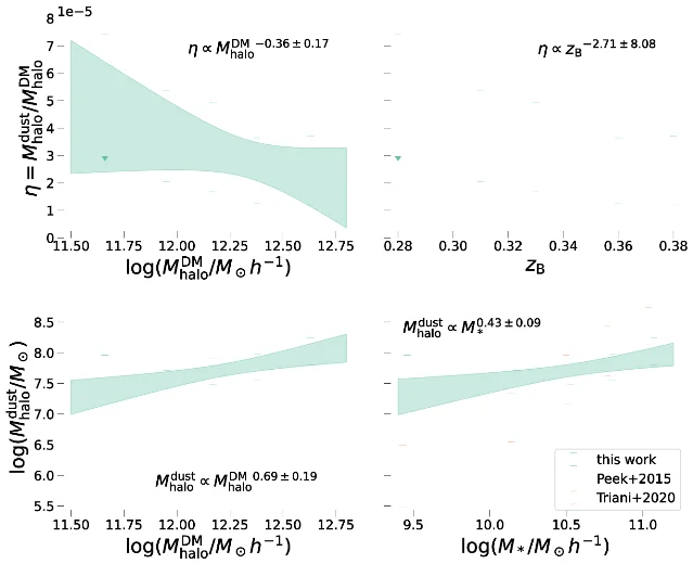
Method and result. The magnitude shift is the point of the paper, because it separates into two terms with different wavelength behaviour: an achromatic magnification term that is a scalar and survives to smaller scales, and a chromatic extinction term from circumgalactic dust. Differencing bands cancels the first and leaves a colour excess that converts to a rest-frame A_V through the Fitzpatrick et al. (2019) extinction curve at R_V = 3.1. Joint modelling of the shear and the four optical bands returns a mean halo mass and a circumgalactic dust mass per bin. Halo masses run from log M_c = 11.66 (+0.12/−0.20) in the lowest bin to 12.63 (+0.12/−0.09) in the highest, all in log(M☉ h⁻¹), and dust masses from log M_d1 = 7.53 (+0.16/−0.27) to 8.02 (+0.09/−0.13). The fits give χ² of 41.9 to 51.2 over 40 degrees of freedom and probability-to-exceed values from 0.11 to 0.39. The scaling relations are the paper's most quotable output: circumgalactic dust mass scales as M_halo^(0.69 ± 0.19) and as M_*^(0.43 ± 0.09), while the dust-to-halo ratio falls as M_halo^(−0.36 ± 0.17). A redshift trend is fitted too, η ∝ z_B^(−2.71 ± 8.08), and the error bar is larger than the exponent, so the redshift dependence is unconstrained.
Real-data stage and caveat. The quoted masses and slopes come entirely from the KiDS shear and magnitude-shift measurements. The MICE2 simulation does not enter the comparison: the KiDS-like mock catalogue of van den Busch et al. (2020) is used to validate the measurement and inference pipeline, with circumgalactic dust injected by hand from the Peek et al. (2015) dust-to-stellar-mass relation and a virial-radius extent. The pipeline recovers the input halo and dust masses within 1σ in every bin except the lowest-mass one, where the dust mass comes back at 2σ, and the probability-to-exceed values stay between 0.05 and 0.95. The only model set against the KiDS data is Dusty-SAGE, which predicts a substantially steeper dust-to-stellar relation than the measurement gives. Caveats the authors state: only mean population properties are measurable, with no scatter; a fixed dust type and a fixed −0.8 radial extinction slope are assumed; the C_s correction for source clustering is approximate; and stellar mass and redshift are degenerate at these depths. The paper also has four internal problems a reader should know before quoting its numbers. Section 5 sends the reader to a "Table 7" for the KiDS best-fit results, but the paper contains five tables and the KiDS fit is Table 5. The lens cut is written z_B < 0.42 in both selection passages and z_B < 0.4 in the abstract and conclusions, and Table 4's top-bin median of 0.41 only survives under the 0.42 version. The fitted magnitude-shift data vector uses the four optical bands while the figures, and the abstract, display all nine. And Section 5 adopts the Fitzpatrick et al. (2019) curve with R_V = 3.1 while Section 7 describes the same assumption as "a fixed SMC-type dust".
Code and data. The paper prints no data-availability statement, no code-availability statement, and no URL at all — there is no
http string anywhere in it. Software is named without links: TreeCorr, emcee, Colossus, LePhare, Bruzual & Charlot templates, BPZ, lensfit and GAaP. The only data-provenance identifiers are the ESO programme IDs for the imaging, 177.A-3016, 177.A-3017, 177.A-3018 and 179.A-2004. 13Why open it. The dust mass is the quantity that decides how much extinction a background sightline accumulates at a given impact parameter, and this is a low-redshift measurement of it over more than 1,300 square degrees, with the chromatic and achromatic halves of the signal separated rather than assumed.
3. Deka et al.: five 21-cm absorbers between z = 0.29 and 0.47, at a rate that matches the local samples
P. P. Deka, N. Gupta, J.-K. Krogager and five colleagues posted H I 21-cm absorption in low- and high-excitation radio-loud active galactic nuclei at z < 0.5 from the MeerKAT Absorption Line Survey on 21 April 2026 at 1:20 p.m. Central Time, and Astronomy & Astrophysics published it online on 28 September, in volume 713 as A319. The journal release is the new event. 3
Sample and observable. The search uses the MeerKAT Absorption Line Survey's L-band data, 900 to 1670 MHz over 391 pointings, cross-matched to SDSS Data Release 18 within 5″ to give 1,965 sources at z < 0.5. Rejecting 57 spurious matches leaves 1,908, of which 613 are classified as radio-loud active nuclei through BPT line diagnostics; a weighted scheme built from five diagnostics splits them into 327 low-excitation and 99 high-excitation radio galaxies. The searched subsample is the 99 sources brighter than 4 mJy at 1.4 GHz — 79 low-excitation and 20 high-excitation — spanning 1.4 GHz luminosities from 10^21.1 to 10^27.0 W Hz⁻¹, with absorption searched within ±2000 km s⁻¹ of the redshifted line. 26
Method and result. Five new absorbers appear, four in low-excitation galaxies and one in a high-excitation one, at emission redshifts of 0.28620, 0.34714, 0.46435, 0.47115 and 0.47290 — all between z = 0.29 and z = 0.47. The uncorrected detection rate is five in 99, about 5%. The paper's headline number is lower: applying a 3σ integrated optical-depth cut of 10.0 km s⁻¹, which leaves 86 sightlines better than the cut, gives 3 (+3/−2) %. Integrated optical depths span 0.27 to 21 km s⁻¹ and the implied neutral columns span 4.9 × 10¹⁹ to 3.7 × 10²¹ cm⁻², under the paper's assumptions of a 100 K spin temperature and a covering factor of 1. The two classes separate in colour: the k-corrected g − r medians are 0.85 ± 0.04 for the low-excitation galaxies against 0.76 ± 0.09 for the high-excitation ones, with a Kolmogorov–Smirnov probability of 3.3 × 10⁻¹⁵. The low-excitation absorbers sit more than 350 km s⁻¹ from the systemic velocity, three of them entirely redshifted and two predominantly blueshifted, which the authors attribute to jet–interstellar-medium interaction or lobe expansion.
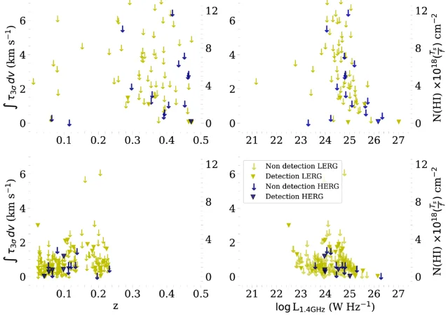
Real-data stage and caveat. The measurement is entirely observational, and no simulation enters any comparison. Instead the paper compares its rate with other surveys at matched sensitivity, which is what the "no redshift evolution" claim rests on: against the WSRT sample of Maccagni et al. (2017), overall 27 ± 6%, and on the 12 sources of this survey matched to that sample's flux and sensitivity, 8.3 (+19.2/−6.9) % here against 20.8 (+4.5/−3.8) % there; against the JVLA sample of Murthy et al. (2021), 19% of 26, and on the subset of both samples better than a 5 km s⁻¹ integrated optical-depth cut, 6.4 (+6.2/−3.5) % here against 15.4 (+12.2/−7.4) % there. The intervals are wide enough that the comparison is a consistency check rather than a detection of evolution. Caveats: five detections, only one of them high-excitation, so no class-dependent kinematics can be compared; the rate is uncorrected for completeness and for the varying optical-depth sensitivity across the sample; the neutral columns assume both a spin temperature and a covering factor of unity, and the paper performs no covering-factor or geometry analysis; 187 of the active nuclei are left unclassified; and the classification rests on hand-chosen weights. Four numerical inconsistencies are worth knowing: the abstract calls 613 sources active while its own Figure 1 caption and Sections 2.4 and 4 say 681; Appendix A quotes 433 narrow-line active galaxies against Section 2.5's 531; Figure 10's caption lists 22 sources split 19 and 4, which sums to 23; and the per-source velocity offsets the text discusses are absent from Table 4, whose velocity column is the 7.1 to 8.1 km s⁻¹ channel resolution.
Code and data. GELATO, the line-fitting code used for the classification, is public on GitHub under GPL-3.0 with 414 commits on its main branch and a newest tag at v2.5.2 from December 2022, which is the version the paper cites. The classified catalogue exists only as the journal's electronic table, and no data DOI is printed for it. The paper points to the MALS data facility at mals.iucaa.in/releases, which is public and states no licence; its description of the first data release as 495,325 sources does not match the 715,760 the paper cites for the same release, and the difference is unexplained in the paper. The journal record itself is carried by Crossref, since the A&A site served an anti-bot challenge on both the article and abstract URLs. 141526
Why open it. It is the highest-redshift sample of its kind and its rate is quoted against sensitivity-matched local samples at the same optical-depth cut, which is the form a low-redshift absorption comparison has to take when the tracer is 21-cm rather than ultraviolet.
4. Anderson et al.: a mock ASPIRE survey returns the same forest statistics for galaxy-biased and random sightlines
Hamish Anderson, Laura C. Keating, Luke Conaboy and three colleagues posted Exploring the influence of reionisation-era galaxies on their local intergalactic medium using the Sherwood-Relics simulations on 22 September at 9:21 a.m. Central Time, and the astro-ph.GA listing carried it on 23 September. No journal reference is reported. 4
Sample and observable. The simulation is a single patchy-reionisation run of Sherwood-Relics: a 160 cMpc h⁻¹ box with 2048³ gas particles, ionising sources placed at haloes above 10⁹ M☉ h⁻¹ with luminosity proportional to halo mass, and ultraviolet background maps built in post-processing with aton. Reionisation ends at z = 5.3. The Lyα forest is drawn along 5,000 periodic sightlines with 78.11 ckpc h⁻¹ pixels, with optical depths from the Tepper-García analytic approximation, and the mock galaxy population is [O III] emitters drawn from haloes at log(M_h/M☉) = 10.55 with a 2.5% duty cycle, giving a comoving number density of 5.78 × 10⁻⁴ (cMpc h⁻¹)⁻³. The mock survey runs over outputs spaced Δz = 0.1 across 5.4 < z < 6.1. 27
Method and result. The mock survey copies the JWST ASPIRE programme's geometry: two 3.62 cMpc h⁻¹ modules separated by a 1.2 cMpc h⁻¹ gap, the quasar sightline placed inside the first module, and the galaxy search capped at 5.83 cMpc h⁻¹. It is repeated 100 times. The statistic is the effective optical depth τ_eff = −ln⟨F⟩ measured in 50 cMpc h⁻¹ bins near the mock emitters, set against a control sample of sightlines at random positions. At a 25 cMpc h⁻¹ influence radius the median Kolmogorov–Smirnov statistic between the biased and random distributions is 0.20, with a 16th-to-84th percentile range of 0.14 to 0.28, and the median p-value is 0.441 with a range of 0.062 to 0.837. A single ASPIRE-sized survey therefore cannot separate the two populations. The paper converts that into a volume requirement: separating them needs about 8,000 cMpc h⁻¹ of sightline at a 5 cMpc h⁻¹ influence radius, roughly four times ASPIRE, and (1.7 to 1.9) × 10⁴ cMpc h⁻¹ at 25 cMpc h⁻¹, roughly ten times ASPIRE. In a separate fixed-snapshot test at z = 6.2, an output outside the survey's own redshift range, the local ionisation field around the mock emitters is about twice the global background and the optical depth drops to 40% of background at r ≈ 6 cMpc h⁻¹.
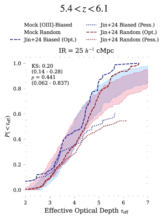
Real-data stage and caveat. Real data enter as an overlay and nothing more. The ASPIRE cumulative distributions of Jin et al. (2024) — 14 quasar sightlines, Lyα forest analysed over the rest-frame range 1040 to 1176 Å, truncated at z ≈ 6.1 — are plotted against the mock distributions, and the abstract's own wording is that the agreement is qualitative. No spectrum is refitted and no χ² is computed. The mock distributions also fail to reproduce the lowest-opacity chunks of the observed data, which the authors attribute to the observed path lengths being truncated at 1040 Å in the rest frame. Caveats the paper states: the source model is not self-consistent and the mock emitters are not realistic; the correlation is computed in real space with peculiar velocities ignored; source clustering cannot be disentangled from geometry by this approach; the 100 cMpc h⁻¹ bin at a 50 cMpc h⁻¹ influence radius approaches the 160 cMpc h⁻¹ box; and a single simulation leaves the modelling uncertainty unquantified. Five internal problems are worth noting. The abstract gives the redshift range as 5.4 < z < 6.2 while the mock survey's own definition, its figures and its conclusions use 5.4 < z < 6.1. The statement that the IGM is more ionised than average at radii between 15 and 50 cMpc h⁻¹ appears only in the abstract and is never restated in the body, which works in influence radii instead. Section 2.2.2 cites Eilers et al. (2018) for the [O III] halo masses while Figure 5 cites Eilers et al. (2024), and the 2018 paper is about IGM opacity, not halo masses. Figure 7 and the text also discuss a z = 6.4 output that lies outside the survey's own 5.4 to 6.2 range. And the fiducial halo-mass cut is written two ways, as log(M_halo/M☉) = 10.55 and as M_halo ≥ 10^10.55 M☉. The paper also contains no table at all, so the gas-particle mass and softening length of the run are not printed anywhere.
Code and data. The paper states that all data and analysis code are available from the first author on reasonable request, and points to the Sherwood-Relics project page. No repository of the authors' own and no dataset DOI are printed. The project's Data Access page describes the simulation data as publicly available and obtained by emailing the two lead investigators, with Lyα forest spectra on cloud storage and a citation request; it prints no self-serve link, no dataset DOI and no licence. The paper's acknowledgements credit p-gadget-3 and aton and disclose the use of ChatGPT for debugging analysis and visualisation code. 1627
Why open it. It turns "current surveys are cosmic-variance limited" into a number on the table — roughly ten ASPIRE-sized surveys to separate galaxy-biased from random sightlines at a 25 cMpc h⁻¹ influence radius — and that number is what decides whether a galaxy–forest correlation measured from any present sample can test a source model.
5. Conaboy et al.: the mock galaxy–forest correlation peaks 10 cMpc inside the measured one, and the realisation scatter is wider than that offset
Luke Conaboy, James S. Bolton, Laura C. Keating and three colleagues posted The impact of source and survey modelling on the connection between [O III] emitters and Lyα forest transmission at z ~ 6 on 2 June 2026, revised it on 28 September at 3:05 a.m. Central Time, and the Open Journal of Astrophysics published it online on 29 September. Both the revision and the release fall inside this week. 5
Sample and observable. The model is built on Sherwood-Relics again, here a 236 cMpc box with 2 × 2048³ particles and a gas-particle mass of 9.41 × 10⁶ M☉, with aton radiative transfer run on a density field refreshed every 40 Myr and sources placed above 10^9.17 M☉. Haloes are populated with [O III] emitters by abundance matching to the Bouwens et al. (2021) ultraviolet luminosity function at z = 5.9, with a 50 Myr duty cycle and a Gaussian relation between the [O III] and ultraviolet luminosities, log₁₀(L_[O III]/L_UV) = −1.42 + 0.49 (log₁₀ L_UV − 10.93), with 0.36 dex of scatter fitted to the luminosity function of Matthee et al. (2023). The mean host halo mass that comes out is 10^10.7 at z = 6. The synthetic observables are the mock [O III] catalogues themselves, the galaxy-to-forest transmission cross-correlation δ_F(r) = ⟨F(r)⟩/⟨F⟩ − 1, the relation between galaxy surface density and effective optical depth, and the projected autocorrelation. 17
Method and result. Two JWST survey geometries are forward-modelled. The ASPIRE case uses five quasar sightlines, a Gaussian distribution of ultraviolet magnitudes with ⟨M_UV⟩ = −19.7 ± 0.7, 7.2 to 10.2 emitters per field across the three redshifts, and 1,024 realisations of the five-sightline sample. The second case follows Zhu et al. (2026): two sightlines, a mosaic with the quasars centred, a luminosity cut at log₁₀ L_[O III] > 42.1, 28 emitters per field and 2,500 realisations per sightline. The measured excess transmission is reported at a separation of about 30 cMpc with an amplitude near twice the global mean, and the mock correlation peaks near 20 cMpc. The paper states that it cannot move the peak from 20 to 30 cMpc within its source model, and that 1 to 2 dex more halo mass would be needed to do it. What stops that being reported as a tension is the scatter between realisations, which runs from 0.3 to 1.6 in the ratio of each realisation's surface density to the mean. On the clustering side, with a luminosity cut at log₁₀ L_[O III] ≥ 42.4 the model's mean is 42.73 at z = 6, which is 0.20 dex above the 42.53 measured by Huang et al. (2026); the paper calls that 1 to 2σ.
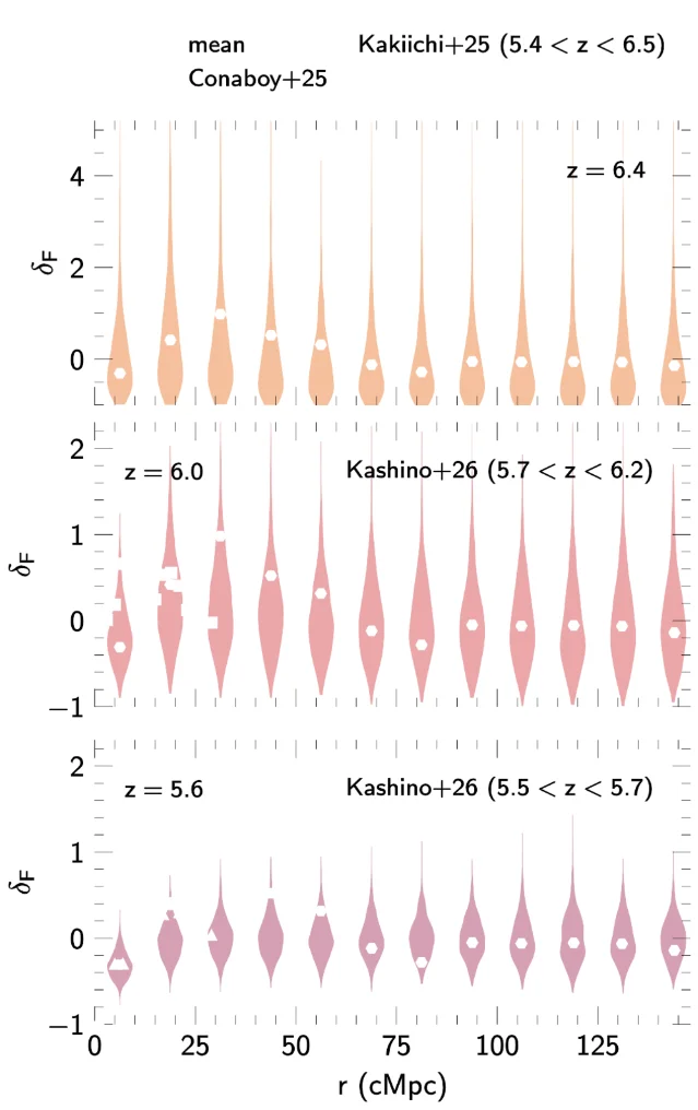
Real-data stage and caveat. The measured luminosity functions, the ASPIRE magnitude distribution and the survey selection cuts enter the model as fitted inputs, and the cross-correlation, the clustering and the surface-density measurements are drawn as overlays and never fitted: there is no likelihood and no χ² against δ_F anywhere in the paper. That is the price of the result, and the authors say so: the mock scatter dominates the comparison, so the model is consistent with the data without being constrained by it. The remaining caveats follow from the setup. The 236 cMpc box is too small for the high-mass end, and the abstract recommends boxes above 250 cMpc while the paper itself uses 236. The one-halo term is missing because haloes are identified with a friends-of-friends finder and one galaxy is placed per halo, which matters below a projected separation of 0.4 cMpc. Module B of the NIRCam pointing, at about 30% of Module A's throughput, is not modelled. And a single late-reionisation source model is carried through the whole paper. Three internal problems: Section 4.4 describes Garaldi et al. (2025b) as both in good agreement with and unable to reproduce the same Ishimoto et al. (2022) point at an effective optical depth of 3; Appendix A sends the reader to Figure 4 for a halo-mass difference of about 0.8 dex that is drawn in Figure 10; and Table 1 gives the Lyα forest extent of the Zhu et al. survey as 74 cMpc while Section 4.2 states the same survey's depth over 5.3 < z < 6.1 as about 370 cMpc. Appendix A also finds that the updated treatment improves agreement with the Lyα emitter and Lyman-break galaxy two-point correlation of Meyer et al. (2020).
Code and data. No repository and no data DOI are printed. The data-availability statement says the paper's data and analysis code are available from the first author on request, and refers readers to the Sherwood-Relics project page, where the simulation data are described as publicly available by email request. The Open Journal of Astrophysics landing page confirms volume 9, the DOI, the 29 September online-publication date and a CC BY 4.0 licence. 1617
Why open it. It is the second attack this week on the same z ≈ 6 galaxy-to-forest statistic, from the source-model side rather than the hydrodynamical side, and it isolates what a mock survey's own source selection and geometry do to the measurement's scatter — the quantity that decides whether the reported excess can discriminate between models at all.
6. Oyarzún et al.: seven damped absorbers with a Lyα-emitting galaxy, and an impact parameter that shrinks with metallicity
Grecco A. Oyarzún, Marc Rafelski, J. Xavier Prochaska and five colleagues posted The KAGG survey: KCWI Analysis of Gas around Galaxies at z~3-5 on 21 September at 1:00 p.m. Central Time, and the listing carried it on 23 September. The paper is accepted for publication in the Astrophysical Journal. 6
Sample and observable. The survey takes 36 damped Lyα absorbers along 17 quasar sightlines, at redshifts between about 2 and 5 and mostly between 3.5 and 4, drawn from the Rafelski et al. catalogues on a single criterion, that the sightline carry at least two absorbers, together with observability. Six nights of Keck/KCWI integral-field spectroscopy between December 2023 and May 2025 give 2 to 5 hours per sightline and 90% completeness at about 4 × 10⁻¹⁸ erg s⁻¹ cm⁻², with a search area reaching an impact parameter of 120 kpc and sensitivity to Lyα luminosities below 10⁴² erg s⁻¹. 28
Method and result. The survey finds 32 significant Lyα emitters, 26 of them within 4,000 km s⁻¹ of a damped absorber, and 7 of those close enough in velocity to the absorber redshift — between −400 and +800 km s⁻¹ — to be called its Lyα emitter, at impact parameters from 14 to 85 kpc. The impact parameters are then tested against metallicity on a composite of 11 emitters: the 7 from this survey plus 4 from the MUSE Analysis of Gas around Galaxies survey, which supplies the large-impact-parameter coverage out to about 300 kpc. The impact parameter falls as metallicity rises, from above 50 kpc at [M/H] near −2 to below 50 kpc at [M/H] near −1, and four emitters within 50 kpc all sit near [M/H] = −1. The significance is the part to read carefully: the Pearson test clears 2σ, but a Monte Carlo over 500 realisations of the survey gives 1.8σ, with the observed slope steeper than 93% of the realisations. A second and wider sample, 35 emitters out to about 300 kpc made of 9 from this survey and 26 from the MUSE sample, shows the same anti-correlation at 2.3σ, which the authors read through the Universe Machine empirical model as a link between DLA metallicity and halo mass. Seventeen further large-scale emitters, found only in this survey, trace overdensities above 5δ and their incidence peaks at [M/H] ≥ −1.5 and z > 4. No Lyα emission is detected from any of the five [C II] emitters that ALMA has found in these fields.
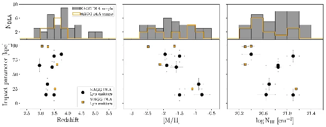
Real-data stage and caveat. No simulation is run and no mock spectrum is generated; the Universe Machine result is an empirical halo model, not a hydrodynamical run. Two caveats govern how far the relation can be pushed. The primary result rests on 11 emitters and on a Monte Carlo significance of 1.8σ against a Pearson result above 2σ, so the relation is tentative by the paper's own accounting. And Lyα is an unreliable indicator of systemic redshift, so the authors can only tentatively call these emitters the damped absorbers' host galaxies, which is why they report the velocity offsets explicitly rather than treating the match as an identification. Five internal problems are worth knowing. Figure 5's caption says the group sample "includes 9 detections" where the text and every other reference give 35. The KCWI field of view is 230 × 140 kpc in Section II.2 and 240 × 150 kpc in the summary. The stated selection of at least two absorbers per sightline fails for two of the sightlines in the paper's own Table 1. Table 1 gives [M/H] = −1.50 for a damped absorber hosting emitters at 14 and 81 kpc, and the 14 kpc emitter contradicts the clean split the paper draws at 50 kpc. And the accepted-at-ApJ status in the comments field has no locator yet, because the related DOI the arXiv record carries, 10.3847/1538-4357/aea982, resolves neither at Crossref nor at doi.org.
Code and data. The paper cites no repository of its own and carries no data-availability statement. The reduction used PypeIt, which is public under BSD-3-Clause with 63 tags and a newest commit on 8 September 2026. One data DOI is printed and resolves: 10.17909/wkh6-0w77, for HST imaging of these damped absorbers. 1829
Why open it. It is the week's clearest galaxy–absorber measurement, and the honest significance — 1.8σ on 11 emitters — is what a reader needs before using the anti-correlation as a prior on where a damped absorber's galaxy sits.
7. Deepak et al.: the cosmic-noon circumgalactic medium is as enriched as today's, and EAGLE puts the enrichment too late
Saloni Deepak, Nicolas Lehner, J. Christopher Howk and three colleagues posted The BRIDGE Survey. I. Metallicities and Physical Properties of Gas Probing the Circumgalactic Medium at Cosmic Noon on 22 September at 12:57 p.m. Central Time, and the listing carried it on 23 September. The paper is submitted to the Astrophysical Journal. 7
Sample and observable. The sample is 105 absorbers selected by their neutral hydrogen column, 16.4 ≤ log N_HI < 20.3, at redshifts from 1 to 2.2, with a mean of 1.81 ± 0.31. By class they are 40 partial Lyman-limit systems, 45 Lyman-limit systems and 20 super-Lyman-limit systems. Selection is blind to metallicity, which is what makes the sample usable for a metallicity distribution. The H I columns come from archival Hubble ultraviolet spectra taken with FOS, STIS, WFC3 and ACS, and the metal lines come from 56 archival high-resolution optical spectra, 30 quasar sightlines with 57 absorbers from one earlier compilation and 26 sightlines with 55 from another. 30
Method and result. Metal columns measured by the apparent optical depth method are fitted against a Cloudy version C13.02 grid inside a Bayesian Markov-chain Monte Carlo, with the HM05 ultraviolet background as the fiducial. The cosmic-noon metallicity distribution has a median [X/H] = −1.19, which is statistically indistinguishable from the −1.18 measured below z = 1 and far above the −2.02 measured between z = 2.2 and 3.6. No absorber falls below [X/H] = −3.5, which the paper reads as an absence of pristine circumgalactic gas at cosmic noon, and a metallicity floor near [X/H] = −2.0 appears for absorbers above log N_HI = 19.0. The plateau is carried by the most diffuse absorbers, between log N_HI = 16.4 and 17.2, which have already reached their z < 1 enrichment level by cosmic noon, while denser absorbers remain more metal-poor than their low-redshift counterparts. Mean N_HI differs by a factor of 400 across the absorber classes while the mean total hydrogen column differs by only 2.5, so the classes differ in ionisation state rather than in total gas content. The absorbers trace overdensities between 400 and 2200, well above the 180 to 500 traced by the KODIAQ-Z sample between z = 2.2 and z = 3.6. Against the EAGLE Recal-L025N0752 run, the observed cumulative metallicity distribution matches the simulation at z = 1 better than at z = 2 even though the sample's mean redshift sits at 1.81, which means the simulated enrichment lags the observations. EAGLE overproduces low-metallicity super-Lyman-limit systems and damped absorbers and underproduces low-metallicity partial and Lyman-limit systems, a pattern the authors attribute to feedback that is too strong and mixing that is too efficient.
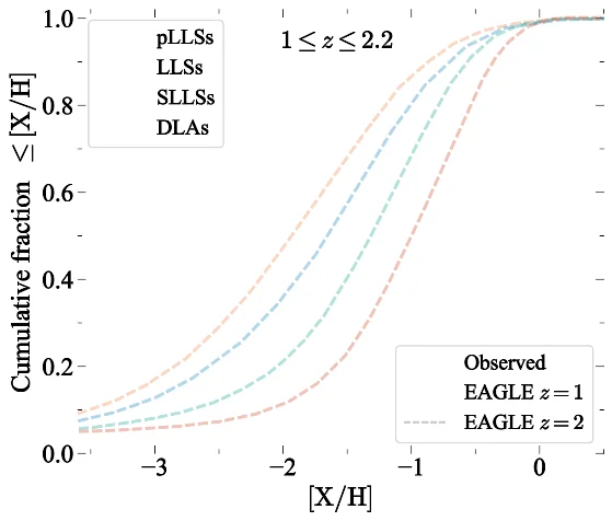
Real-data stage and caveat. No mock spectra are produced and no new mock absorbers are generated; the simulation enters only as the published EAGLE cumulative distributions at two redshifts, which makes this a benchmark at the level of physical quantities rather than a spectrum-to-spectrum comparison. Three caveats matter. The fit assumes the HM05 background is the right one, and switching to the HM12 background moves the result by 0.16 ± 0.13 dex, which is the size of the background-model systematic on this metallicity scale. A Hartigan dip test finds no bimodality in any class, so the distribution is not resolving into two populations. And the sample bookkeeping is loose in a way that matters for anyone reusing the catalogue: the abstract and two of the tables quote 105 absorbers, one table's row for this sample reads 80, a fourth table lists 100 rows, and five absorbers in the sample table sit below the stated log N_HI floor of 16.4. The paper's own comments field says 29 figures where the document has 23 numbered ones.
Code and data. Two public tools underlie the analysis: pyigm, public with no licence file and a newest commit on 5 December 2022, and rongmon/rbcodes, public under MIT with a newest commit on 16 September 2026. The paper says 26 Keck/HIRES spectra will be uploaded to the KODIAQ database and that all its tables are available in machine-readable format, but it prints no address or DOI for either, and carries no data-availability section at all. 1920
Why open it. It is the metallicity benchmark a simulated circumgalactic medium has to match at cosmic noon, and the EAGLE comparison shows the failure mode a mean metallicity would hide: a redshift offset between simulated and observed enrichment, visible because the sample's mean redshift sits between the two simulation outputs.
8. Poudel et al.: the LMC's wind thins out 125 to 200 kilometres per second outflowing, and the fast gas is not all the Cloud's
Suraj Poudel, April Horton, Kathleen A. Barger and 22 colleagues posted Tracing Winds through the Fog: A Comprehensive Survey of LMC's Galactic Outflows with ULLYSES on 25 September at 8:48 p.m. Central Time, and the listing carried it on 29 September. The paper is accepted for publication in the Astrophysical Journal. 8
Sample and observable. The background sources are 170 OB stars from ULLYSES Data Release 7, which holds 182 sightlines through the Large Magellanic Cloud; 12 were dropped for complex continua, low signal-to-noise or missing line coverage. The Cloud sits 50 kpc away and is nearly face-on at an inclination of 23.4°, so each sightline passes through its disk and its outflow before reaching the star. Eighty-nine sightlines have STIS/E140M spectra at 6.5 km s⁻¹ resolution and the rest COS at 17 km s⁻¹, 44 also have STIS/E230M and 86 have FUSE, and continuum signal-to-noise per resolution element runs between 20 and 30. Silicon II is covered along 165 sightlines, O I along 156 and S II along 150. 31
Method and result. Voigt-profile fits with VoigtFit 3.14.1.1 are performed across multiple transitions of each ion at once, with an apparent-optical-depth analysis supplying lower limits and fixed-window integrated columns where components are saturated. The mean Si II column density falls steadily out from the disk and reaches a minimum between v_LMCSR ≈ −200 and −125 km s⁻¹, which marks the boundary between a denser slow wind and more diffuse fast material. The bulk wind runs from −30 to −100 km s⁻¹ relative to the Cloud, and the fastest components reach −175 km s⁻¹. Fitting the slow wind gives log N(Si II) = 0.013 (v_LMCSR/km s⁻¹) + 15.16 with 0.58 dex of residual scatter; of the 349 components inside the ambiguous velocity window, 190 follow that trend and 159 sit above it by a median 0.5 dex, with no statistically distinct split into two populations. Comparing with star-formation-rate surface density from Hα, the slow gas shows a weak but statistically favoured positive correlation and the −200 to −100 km s⁻¹ gas an apparent negative one, which the authors caution is driven by large scatter. Cloudy 25.00 modelling of 13 selected sightlines, with a composite radiation field combining the Milky Way disk, the Magellanic Clouds and the extragalactic background, gives [O/H] between −0.9 and −0.2, silicon depletion between −0.5 and +0.3, and cloud distances from 3.7 to 8.3 kpc from the Cloud. Of 19 modelled Si II components, 12 fall near the observed column-velocity trend and 7 sit above it, and the chemistry does not map cleanly onto that split.
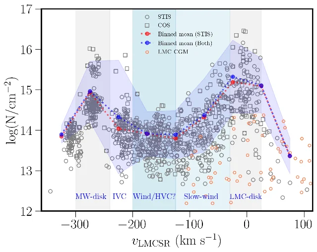
Real-data stage and caveat. No cosmological simulation enters the comparison; the modelling is radiative transfer through Cloudy. The central caveat is contamination, and it is large. Gas between roughly +90 and +175 km s⁻¹ in the local standard of rest overlaps the Milky Way's high-velocity clouds, and the paper concludes that this fast gas likely mixes three origins: LMC-driven wind, Magellanic-associated high-velocity clouds and foreground Milky Way gas. Metallicity, dust depletion, spatial association and kinematic continuity together do not separate them, and the authors note that some unambiguous Milky Way high-velocity clouds also show high metallicity and depletion. They identify the clean test as absorption towards Milky Way halo stars at known distances, and place it outside the scope of the paper. Four further inconsistencies are worth noting: the abstract puts the Si II minimum at −100 to −200 km s⁻¹ where Section IV.1 puts it at −200 to −125; the ambiguous velocity window is quoted three different ways across the paper, as +90 to +175, +100 to +175 and, in the abstract and summary, +100 to +150; the regional outflow masses in the text disagree with Table 5 for both the leading and trailing sides; and the comments field describes three tables where the paper has five. GIZMO appears in the software list but nowhere in the body, so its role cannot be checked.
Code and data. The paper provides the normalised and unnormalised spectral snippets for every sightline and fitted transition through a public GitHub repository, which is public with no licence, no tagged releases and a most recent commit on 25 September 2026. The radiation-field tool galrad is public under BSD-3-Clause with a last commit in June 2022. The ULLYSES data carry the MAST DOI 10.17909/T9-JZEH-XY14, which resolves. One printed archive address, the Milky Way H I survey at the University of Bonn, returned an HTTP 403 from this run and its content could not be verified. 213233
Why open it. It is the largest down-the-barrel ultraviolet absorption sample in existence, and its contamination problem is the same one a simulated galaxy wind has to solve before a mock column can be set beside an observed one: which of the components along the line of sight actually belongs to the galaxy in question.
9. Mangola et al.: ninety per cent of metal lines found at a line signal-to-noise of four, and every confident mistake sits beside a damped absorber
Elena Sofia Mangola, Francesco Pistis, Michele Fumagalli and seven colleagues posted Detection of metal absorption lines in quasar spectra: a neural network approach using U-Net on 23 September at 8:18 a.m. Central Time, and the listing carried it on 24 September. The paper is accepted in Astronomy & Astrophysics. 9
Sample and observable. The training set is 50,000 mock quasar spectra built to the WEAVE-QSO survey specification over the rest-frame interval from 1230 to 3095 Å at 0.114 Å spacing, with quasar redshifts from 2.1 to 4.8, absorber redshifts from 0.2 to 4.8, neutral hydrogen columns from 17 to 22.5 in log N_HI and twelve metal ions injected: O I, C II, Al II, Zn II, Si IV, C IV, Ni II, Mn II, Mg II, S II, Fe II and Si II. The Lyα forest comes from a lognormal real-space density field, the noise is flux-dependent at an air mass of 1.107 with a sky brightness of 20.92 mag arcsec⁻² and includes atmospheric skylines, the line-spread function corresponds to a resolving power of 5,000, and the continuum is a principal-component model normalised to unity. Because the network is fed the rest-frame wavelength array, the analysis is redshift-independent by construction. 34
Method and result. The detector is a one-dimensional U-Net with encoder, decoder and skip connections, trained with a weighted sparse categorical cross-entropy on about 35,000 of the 50,000 spectra, with the rest split between validation and test, and its hyperparameters chosen by a Bayesian search over 50 trials. On the held-out 7,500 spectra with an ideal continuum, completeness, purity and F1 all reach about 90% at a line signal-to-noise of 3.80 and 100% at a line signal-to-noise of 8. Aggregated over every line retained for training, F1 is about 82%, completeness 92% and purity 74%. Line centres are recovered with a mean offset of −0.028 Å and 0.205 Å of scatter, with 73.5% of detections inside one pixel and 49.7% inside half a pixel. Repeating the detection after an autoencoder reconstruction of the continuum, which is how the authors simulate the continuum-fitting step real data require, changes F1 by less than 10% above a line signal-to-noise of 3 and by about 5% at 4. The false-positive result is the one to carry away: 17 false positives survive above a line signal-to-noise of 5, and all of them sit near damped Lyα features, at an average separation in redshift of 0.015 between the quasar and the damped absorber.
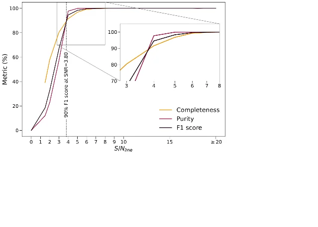
Real-data stage and caveat. The network never sees a real survey spectrum. Every number is measured on mock data, and the real-data validation belongs to a companion paper that applies the pipeline to DESI Data Release 1 and finds its C IV detections in 1.2σ tension with existing catalogues; that companion is not this paper. Four caveats follow. The mocks are WEAVE-like rather than WEAVE, and the WEAVE-QSO specification quoted covers quasars at z ≥ 2.2 while the mocks start at 2.1. The training labels keep lines above a line signal-to-noise of 1.5, so what the network is being asked to find is defined by a threshold the authors chose. The false-positive result above a line signal-to-noise of 5 is a count of 17 rather than a rate, and the paper prints no fractional false-positive rate at any threshold; the counts in the relevant figure fall to one or two per bin above 5. And the noise model assumes a fixed air mass and sky brightness, so a survey observed in worse conditions is not represented. The largest internal problem is that Table 4 prints F1, completeness and purity of about 99% at a line signal-to-noise of 4 where Figure 4 shows about 90% at the same value — reconcilable only if the table is cumulative over a different threshold, which the paper does not state. The abstract and Section 4.1 also differ on whether the false-positive threshold is at or above a signal-to-noise of 5.
Code and data. The paper names no code repository and prints no data-availability statement. It does print one DOI, 10.5281/zenodo.22711575, which resolves to a Zenodo software record carrying the trained autoencoder and U-Net weights, 207.8 MB and 1.3 MB, published on 11 September 2026 under CC BY 4.0. A Zenodo deposit is a single immutable version rather than a repository, so there is no commit history and no tagged release to inspect, and no claim can be made here about any analysis code beyond the trained models. 22
Why open it. It is the cleanest performance curve for automatic metal-line detection published this week, and the false-positive finding is the part to carry into a real search: every high-significance mistake this network makes is a damped absorber being mistaken for the lines around it, which is exactly the region where a metal-line catalogue is hardest to trust.
10. Karam et al.: a frozen image model reads cooling time off a mock X-ray image and keeps 0.50 dex when the simulation changes
Rawan Karam, Carter Lee Rhea, Julie Hlavacek-Larrondo and four colleagues posted Cool Embeddings: Predicting Galaxy Cluster Cooling Times in IllustrisTNG and TNG-Cluster with AstroCLIP on 26 September at 7:57 a.m. Central Time, and the listing carried it on 29 September. The paper is submitted to the Astrophysical Journal. 10
Sample and observable. The input is mock Chandra ACIS-I images, 252 × 252 pixels, one channel, three orthogonal projections per cluster, generated from IllustrisTNG snapshot 99 at z = 0 with a particle-to-photon X-ray simulator. Gas cells inside one R_500 are rendered with single-temperature APEC spectra, a Galactic column of 4 × 10²⁰ cm⁻², photons between 0.5 and 10 keV reduced to a 0.5 to 7.0 keV band, the Cycle 19 ACIS-I response and on-axis point spread function, 200 ks of exposure, and instrumental and astrophysical backgrounds included. Point sources are detected and filled before analysis. The sample is 237 clusters from TNG300 giving 711 images and 331 from TNG-Cluster giving 993. The target quantity is the central cooling time of the intracluster medium, log t_cool,0, measured inside a three-dimensional radius of 0.012 R_500c, which is a quantity traditionally obtained from X-ray spectroscopy. 23
Method and result. Embeddings from the frozen AstroCLIP vision-language model, which was trained on optical galaxy images and spectra, are used unchanged as 1,024-dimensional features, and four regressors are compared. The best is a retrieval model that takes the ten or fifteen nearest training clusters in embedding space and reweights their cooling times by scaled dot-product attention. Its root-mean-square error is 0.24 dex on TNG300 and 0.23 dex on TNG-Cluster, against 0.38 to 0.49 dex for the multi-layer perceptron, residual network and plain attention baselines, and 0.59 dex on the merged set against 0.74 to 0.76 for the baselines. The paper also reports a training-free baseline that averages the four nearest neighbours and discards the worst, which gives 0.55, 0.59 and 0.83 dex. The informative number is the transfer test: trained on TNG-Cluster and evaluated on TNG300, the retrieval model holds 0.503 dex where a convolutional network fine-tuned for the task gives 0.729 dex and collapses towards a nearly constant prediction. The embeddings also carry physically meaningful structure without being told to — clusters with similar thermodynamic properties group together in the latent space, and halo mass does not produce an equivalent separation.
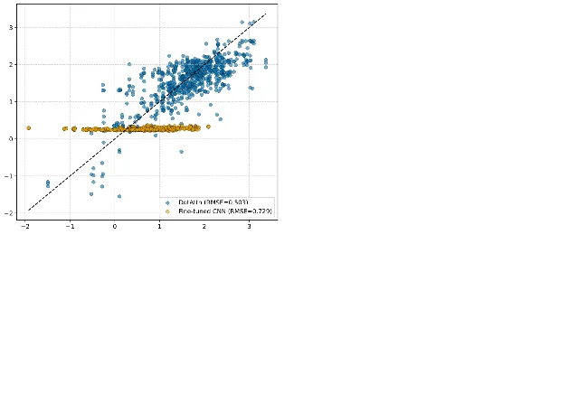
Real-data stage and caveat. Every image in the training set, the validation set and the test set is simulated. No real X-ray image enters anywhere, and the paper says plainly that it remains to be determined whether the performance extends to real observations. The only real ingredients are the instrument response, the background models and the Galactic column. The transfer test varies the simulation, but both simulations are IllustrisTNG and therefore share the same subgrid physics, so what the test measures is a change of volume and cluster population rather than of feedback model. The other caveats are ordinary: the target is the cooling time at a single cosmological epoch, the projections are only three per cluster, and the embeddings come from a model trained on optical data, which is a substantial change of modality and physical scale. Four internal problems are worth knowing. Section II.1 quotes 280 most-massive TNG300 haloes where Section II.3 uses 237, and the TNG-Cluster count drops from 352 to 331 with no explanation. Figure 4's mass bins and class counts sum to 714 images against the stated 711. Figure 5's caption carries Figure 6's out-of-distribution numbers. And the Data Availability section prints the MNRAS template text with no statement at all, although the arXiv comment says the paper was submitted to the Astrophysical Journal.
Code and data. No repository of the authors' own is named. The only GitHub links in the paper belong to the third-party simulators pyXSIM and SOXS, and this run did not open either, so nothing can be said here about them. No data DOI and no archive address are printed for the mock images or the embeddings, and the Data Availability section is boilerplate rather than a statement. 23
Why open it. It puts a number on the transfer question that any model trained on a single simulation has to answer: retrieval keeps 0.50 dex of scatter when the simulation underneath it changes, where a fine-tuned convolutional network gives 0.73.
11. Abghari et al.: a scattering transform, a public package, and one Planck map that sits above every simulated sky
Arefe Abghari, Lukas T. Hergt, Douglas Scott and Raelyn M. Sullivan posted HierArchical Wavelet Coefficients on the Sphere (HAWCS): the Scattering Transform on Spherical Maps on 21 September at 8:22 p.m. Central Time, and the listing carried it on 23 September. No journal reference is reported. 11
Sample and observable. The objects are full-sky maps in HEALPix format. The summary statistic is a wavelet scattering transform taken to second order: a mean term, the mean of the modulus of the map filtered at one scale, and the mean of the modulus of that modulus filtered at a second, strictly larger scale. At ten dyadic scales that is 56 coefficients, from the formula 1 + J + J(J−1)/2. The quantity the paper actually plots is an excess over matched Gaussian control maps, which share the power spectrum, beam, noise and mask of the map under test, so the statistic isolates non-Gaussian structure rather than the power spectrum. 35
Method and result. The package is built on the healpy convention with a Morlet-like axisymmetric wavelet in real space, and its cost scales as the cube of the maximum multipole against the fifth or sixth power for a bispectrum and up to the tenth for a trispectrum; the paper prints these scalings and no wall-clock timing, so the efficiency claim rests on the exponents alone. Validation on quadratic non-Gaussian fields reproduces the expected growth with the non-Gaussianity amplitude. The application is to the Planck 2015 thermal Sunyaev–Zel'dovich y maps in the MILCA and NILC reconstructions, at first-layer scales of 18.3, 36.6, 73.3 and 146.6 arcmin, against simulated y maps from Websky, a rescaled Sehgal et al. (2010) realisation used in Simons Observatory forecasts, Magneticum, and HalfDome, the last with eleven fixed-cosmology realisations. Read off the panels, the excess runs from about 0.021 to 0.039 for MILCA, 0.008 to 0.020 for NILC, and 0.005 to 0.042 across the four simulations. MILCA exceeds every simulation at every scale tested, and no simulation reproduces the two-scale dependence that either Planck map shows. The scatter across the eleven HalfDome realisations is smaller than several of the differences between simulations, and smaller than the MILCA-to-NILC difference, which the paper takes to mean those differences are not cosmic variance alone.
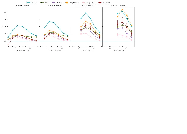
Real-data stage and caveat. Real Planck maps are set against simulated maps, which places this in the same class as the two Lyα forest comparisons above. The caveat is that the comparison is presented only in figures: no χ², no p-value, no fitted amplitude and no tabulated coefficient appears in the text, and the values quoted here are read off a verified-legible panel. The paper also prints no redshift, no resolution and no cosmology for any map it compares, because the application is a full-sky projection rather than a redshift-binned measurement. A second application, to a simulated CMB temperature map rather than a real one, carries the paper's own caution that its deviations should not be interpreted as independent or as a joint detection at a stated significance, although no printed coefficient or error bar in the paper supports a deviation of that size. The Data Availability section is printed empty even though the introduction describes the package as open-source.
Code and data. The package is public on GitHub under an MIT licence, and it sits on the repository's
master branch. That branch holds eight commits, with a most recent commit on 18 September 2026, and carries no tagged releases; the package has no PyPI entry. Two structural problems are worth knowing before anyone tries to install it: the repository's default branch is main and is empty, so a visitor who follows the repository link lands on nothing, while the link the paper itself gives points to master; and the project metadata points its own URL field at a repository path different from the one the paper cites. No data DOI or archive address is printed for the Planck maps or for any of the four simulations. 24Why open it. It is a working, licensed and freshly updated summary statistic for full-sky maps, and its tSZ result is a warning about how validation is usually done: one of the two standard Planck reconstructions sits above every simulated sky the paper could put beside it, at every scale, and the eleven-realisation scatter is too small to explain that.
What the eleven items change in a comparison pipeline
The eleven items bear on four separate pieces of the route from a simulation to a measured quantity.
- What the detection step removes before the comparison starts. The DESI sodium search can only claim half the absorbers at a rest equivalent width of 0.95 Å, and its ×3.4 rise rests on the 1,336 of 3,636 doublets above that floor; the U-Net in mock survey spectra reaches ninety per cent on all three metrics only at a line signal-to-noise of four, and every one of its high-significance false positives lands near a damped absorber; the MALS 21-cm rate falls from five per cent raw to three per cent once a 10 km s⁻¹ optical-depth cut is applied. Any of these numbers quoted without its floor is a different number. 252634
- Whether a survey is large enough to test a source model. Anderson et al. put the Kolmogorov–Smirnov p-value between galaxy-biased and random sightlines at 0.441 for one ASPIRE-sized mock survey, and the requirement for telling them apart at roughly ten ASPIRE volumes for a 25 cMpc h⁻¹ influence radius. Conaboy et al. show the other side of the same coin, where the realisation scatter among mock survey measurements is wider than the offset between the mock and measured correlation peak, so a model is called consistent with the data without being constrained by it. Together these two set the sample size at which a galaxy-to-forest measurement stops being an upper limit on model space. 1727
- A significance quoted against a resampling test as well as against a coefficient. The KAGG relation between impact parameter and metallicity clears 2σ on a Pearson test and 1.8σ on a Monte Carlo over 500 realisations of the survey, on 11 objects. The distance between those two numbers is the honest measure of what the relation will do as more emitters are added. 28
- The simulation's own assumptions are where the disagreement sits. EAGLE matches the observed cosmic-noon metallicity distribution better at z = 1 than at z = 2 although the sample's mean redshift is 1.81, and overproduces low-metallicity super-Lyman-limit systems while underproducing low-metallicity Lyman-limit systems — a pattern that a single median metallicity would not reveal. The AstroCLIP transfer test shows what happens when the underlying simulation changes rather than the task: retrieval holds 0.503 dex where a fine-tuned network gives 0.729. 2330
Three tests follow for anyone assembling one of these comparisons.
First, before putting a mock observable beside a measurement, write down the completeness floor and the purity of the measurement and check that the mock's own detection step would produce the same floor. The 0.95 Å sodium boundary and the line signal-to-noise of four in the mock spectra are both properties of a pipeline, and a simulation compared with an absorber catalogue that has a different floor is being compared with a different sample.
Second, if the statistic is a correlation between galaxies and forest transmission, compute the realisation scatter before computing the offset. When a peak sits 10 cMpc from the measured one and the scatter across realisations spans a factor of five in normalisation, the offset is smaller than the uncertainty on it, and the useful output of such a run is the survey volume at which the two become distinguishable.
Third, when a mock catalogue is used to calibrate a measurement rather than to test it, keep the two roles apart in the write-up. The KiDS dust analysis uses its simulation only to show that the pipeline recovers injected halo and dust masses within 1σ, and that holds in every mass bin except the lowest one, where the dust mass comes back at 2σ; the only model set against the data is a semi-analytic one, and a reader who treats the simulation as a comparison partner will over-read what the paper claims.
Coverage note
This issue covers the arXiv announcement days of 23, 24, 25, 28 and 29 September 2026, together with items whose journal online publication falls on those dates. Items admitted on or before the 22 September announcement day are excluded, because the previous issue closed on that day. The weekly listings returned 170 astro-ph.GA, 120 astro-ph.CO and 85 astro-ph.IM entries across those five days, which covers what those days announced rather than everything submitted in the window. 363738
Two of the eleven entered on a journal release, and both dates come from the publishers' own records. The Open Journal of Astrophysics published Conaboy et al. on 29 September, confirmed on its landing page, which also gives volume 9 and a CC BY 4.0 licence. Astronomy & Astrophysics published Deka et al. online on 28 September in volume 713 as A319, confirmed through the Crossref registry record for DOI 10.1051/0004-6361/202660447; the journal's own site served an anti-bot challenge on both the article and abstract pages, so that date rests on the deposited record rather than on a page read directly. 35
A sweep of journal online publications dated 23 to 29 September through Crossref covered 21 astronomy journals. The Astrophysical Journal and its Letters, the Astronomical Journal, MNRAS, Astronomy & Astrophysics, PASP, JCAP, Nature Astronomy and Research Notes of the AAS returned 394 records between them, and twelve further journals about 30 more. Seven of those records were close enough to pull in full. Two are carried above, as Deka et al. and Conaboy et al. One is a release this channel has already covered: the Astrophysical Journal published Trevino et al. online on 29 September, and that paper's preprint was one of the five items in the 8 September issue, so the release is not carried again here. The remaining four were set aside as secondary to the eleven: a jet-aligned Hα study of the cool circumgalactic medium with a Mg II counterpart along the same DESI sightlines, a 21-cm emission study of the inner haloes of NGC 891 and NGC 4565, a convolutional network for Galactic H I self-absorption, and a diffusion emulator for 21-cm lightcones. 39
No paper in this window generates Lyα forest spectra from a cosmological simulation and fits them to observed low-redshift forest spectra. The two items closest to that description both work at z ≈ 6: Anderson et al. compare their own mock τ_eff distributions with the ASPIRE measurement without fitting anything, and Conaboy et al. overlay their mock galaxy-to-forest correlation on the measured one without a likelihood. Two further in-window candidates were screened and left out of the eleven because their subject sits away from the route this channel follows: a random-forest classifier over FIREbox haloes that separates recently ignited haloes from starless ones at an area under the curve of 0.823 once the halo's own neutral-gas reservoir is included, and a convolutional network that detects Galactic H I self-absorption in 21-cm spectra at 96.5% accuracy and 97.0% recall on synthetic data. 1727
References
- 1
- 2
- 3
- 4
- 5
- 6Oyarzún et al., The KAGG survey
arxiv.org
- 7Deepak et al., The BRIDGE Survey I
arxiv.org
- 8
- 9
- 10Karam et al., Cool Embeddings
arxiv.org
- 11Abghari et al., HAWCS
arxiv.org
- 12qsoabsfind
github.com
- 13Genc et al., full text
arxiv.org
- 14GELATO
github.com
- 15MALS data releases
mals.iucaa.in
- 16Sherwood-Relics data access
nottingham.ac.uk
- 17Conaboy et al., full text
arxiv.org
- 18HST imaging of the KAGG DLAs
doi.org
- 19pyigm
github.com
- 20rbcodes
github.com
- 21LMC_Winds
github.com
- 22Trained networks on Zenodo
doi.org
- 23Karam et al., full text
arxiv.org
- 24HAWCS repository
github.com
- 25Anand & Muzahid, full text
arxiv.org
- 26Deka et al., full text
arxiv.org
- 27Anderson et al., full text
arxiv.org
- 28Oyarzún et al., full text
arxiv.org
- 29PypeIt
github.com
- 30Deepak et al., full text
arxiv.org
- 31Poudel et al., full text
arxiv.org
- 32galrad
github.com
- 33ULLYSES data on MAST
doi.org
- 34Mangola et al., full text
arxiv.org
- 35Abghari et al., full text
arxiv.org
- 36
- 37
- 38
- 39Trevino et al., arXiv:2609.04324
arxiv.org
This story was produced automatically by a channel. One sentence is all it takes for Neodrop to keep producing for you.