Twelve gas-census updates: 17 to 28 per cent of the baryons inside halos, a WHIM tracer excess of 2.6, and two 21-cm absorbers 0.035 apart in redshift
Twelve papers turn on one step, the conversion between what an instrument records and the quantity a model predicts, and this issue reads the week's new low-redshift absorption, baryon-budget and spectral-emulation results for how far that step moves the answer.

Twelve papers this week, and most of them turn on one step: the conversion between what an instrument records and the quantity a model predicts. That step takes different forms here — a colour into an H I mass, an optical depth into a column density, two equivalent widths into a lower bound, a galaxy field into a gas field — and several of the week's results are about how far the step moves the answer. The scale it operates at shows in one comparison: three cosmological simulations leave 72 to 83 per cent of the cosmic baryon budget outside halos at redshift 0, and the intergalactic fraction inferred from localized fast radio bursts ranges from 0.59 to 0.93 across four published analyses, from eight sightlines with spectroscopic foregrounds up to a 17-burst sample. 12
The absorption measurements in the same week do the same arithmetic on gas near galaxies, and their answers turn on the same kind of conversion. A MUSE-ALMA census weighs the condensed baryons of 79 galaxies selected by the H I absorbers in front of them, and its two H I mass estimators agree only where the impact parameter is small. 3 A MeerKAT sightline turns two optical depths into two column densities through an assumed spin temperature and covering factor. 4 Two method papers work on that step directly, one from two equivalent widths alone and one by emulating a radiative-transfer library until it can be fitted against real spectra. 56
Four of the twelve items set a synthetic observable against a measured counterpart of that same quantity, and each of the four reports how much of the agreement or disagreement follows from the way the synthetic side was built. One item benchmarks a simulation against analytic models of the same gas with no data in the comparison, and one is synthetic-only, validated against held-out simulation truth. The remaining six report measurements on real absorption data, and five of them work below z = 1.3.
The order below puts the low-redshift measurements first, then the conversion step that entry 5 supplies, then the week's broadest stack, the simulation-side accounting, and the two synthetic-spectrum comparisons last.
Quick look
The class in each row reads as follows: (a) a synthetic observable set against a measured counterpart of that same observable, where the synthetic side comes from a hydrodynamical simulation, a radiative-transfer model or a forward model; (b) a simulated result set against an analytic or theoretical model of the same gas, with no data in the comparison; (c) a synthetic-only result, with no observed counterpart of the synthetic observable in the comparison; (d) a measurement, or a measurement method, applied to real absorption data, with no synthetic observable in the comparison, where a simulation may still stand behind the interpretation.
| Work | Class and redshift | Comparison level | Result to screen on | Code and data |
|---|---|---|---|---|
| O'Beirne et al., arXiv:2610.10117 | (d) observational anchor; sample at 0.2 < z < 1.2, absorbers up to z = 1.2 | 79 galaxies near 32 H I absorbers on 19 quasar sightlines, with H I masses inferred two ways and TNG50 tracks for the same stellar-mass range | The two H I mass estimators agree within their scatter for impact parameters below about 100 kpc and diverge in group environments; d log(M_H I/M*)/d log M* = −0.50 ± 0.05 against −0.88 ± 0.08 for H₂ 3 | No repository, dataset DOI or catalogue is named anywhere in the paper 7 |
| Péroux et al., arXiv:2610.10112 (A&A 708, A146) | (d) survey data release; 39 galaxies at 17 absorbers, z ≈ 0.5 | 61.5 hours of ALMA Cycle 10 on H I-absorption-selected galaxies, with the reduction choices and the achieved sensitivity printed for the release | Continuum RMS of 173 to 492 µJy per beam and a design sensitivity of log M_H2 > 9 M⊙ at 5σ; self-calibration gains a factor of 1.1 to 7.6 8 | ALMA programme 2023.1.00127.L; raw data in the ALMA Science Archive; combined cubes at the survey page 9 |
| Martínez-Acosta et al., arXiv:2610.11203 | (d) observational anchor; 0.1 ≤ z ≤ 0.5 | Ten HST/COS sightlines against 22 independent cluster-pair systems, compared with the survey's own field expectation | Broad Lyα absorbers at 2.3 (+0.9/−0.7) and O VI at 2.6 (+1.3/−0.9) times their field incidence, at 2.0σ and 1.8σ 10 | Table 3 is deposited at CDS; the HST programmes are GO 12958 and GO 15293 11 |
| Mohapatra et al., arXiv:2610.07273 | (d) observational anchor; z = 0.5305 and 0.56530 towards one blazar | One MeerKAT sightline, with SDSS and DESI spectra for the metal lines | Integrated optical depths of 0.31 ± 0.04 and 1.31 ± 0.04 km s⁻¹, column densities of 10^19.75 and 10^20.37 cm⁻², and a redshift separation of 0.0348 4 | No data-availability statement; raw visibilities in the SARAO archive under project SCI-20180516-NG-01 12 |
| Badash & Kushnir, arXiv:2608.04088 (MNRAS, online 9 October) | (d) measurement method; local and host-galaxy sightlines | 36 published Na I D sightlines used as the test set | A certified lower bound on the column density, within 0.08 dex of the profile-fitted value for doublet ratios above 1.4 and conservative by a factor of 3.5 at 1.1 5 | A reference implementation at github.com/DoronKushnir/doublet_inversion, with Table 2 as machine-readable data 13 |
| Napolitano et al., arXiv:2512.02992 (AJ 172, 250, online 7 October) | (d) observational anchor; 0.287 < z_abs < 2.505 | 239,174 DESI DR2 quasar spectra with one Mg II absorber each, against a 2,061,617-spectrum matched control | A 72-line composite atlas with Lyα at W₀ = 9.750 Å and Mg II 2796 at 1.873 ± 0.001 Å; [O II] needs about 10,000 stacked spectra to resolve 14 | Figure data and catalogue released on Zenodo; no code repository 15 |
| Ayromlou et al., arXiv:2610.07140 | (a) synthetic observable against measured; z = 0, simulation curves to z = 5 | TNG100, EAGLE and SIMBA with matched dark-matter-only runs, against published halo baryon fractions and FRB-derived IGM fractions | Baryons inside halos at 17, 21 and 28 per cent at z = 0; closure envelope of 1.8 to 6.4 cMpc; the compensation wavenumber matches the power-spectrum recovery scale to within 2 per cent 1 | PROFI on GitHub; all three simulations public; derived products on request 16 |
| Rufo-Pastor et al., arXiv:2610.08931 (MNRAS, online 10 October) | (b) model benchmark; z = 0 to 5 | Six VINTERGATAN-GM zoom runs against an analytic virial-shock model and the TNG mass-growth distribution | A hot corona at the virial radius from z ≈ 4 with feedback and near z ≈ 1 without it; the virial-shock model reaches shock stability only at z ≲ 1.5 17 | IllustrisTNG data at tng-project.org; VINTERGATAN products on request 18 |
| Konietzka et al., arXiv:2507.07090 (ApJ 1010, 122, online 12 October) | (a) synthetic observable against measured; z = 0 to 5.5 | Ray-traced TNG300-1 sightlines against observed FRB dispersion measures over z ≤ 1.25 | The trapezoidal integration used in earlier TNG work moves the dispersion-measure width by more than 50 per cent; a two-parameter modified normal fits every redshift slice 19 | More than 20 public dispersion-measure catalogs; code on request 20 |
| Hussaini et al., arXiv:2610.10741 | (c) synthetic-only; z = 0 | CAMELS50 (IllustrisTNG), 980 training boxes of 50 h⁻¹ Mpc, validated against held-out simulation truth | Per-sightline dispersion measure scatter of 0.193 dex at a best-fit slope of 0.81; a low-feedback reconstruction is wider than a high-feedback one by 0.0163 ± 0.0020 dex 21 | No code or data statement in the paper 21 |
| Wallis et al., arXiv:2610.07364 | (a) synthetic observable against measured; nova-like cataclysmic variables | 88,680 Sirocco spectra emulated and then fitted to five HST/STIS spectra, three of them shown | Emulator samples of 1.66 to 37.48 ms against 1 to 2 CPU-core-hours per direct Sirocco run; inclination is the worst-calibrated parameter at 26 per cent coverage in 1σ 6 | github.com/sirocco-rt/speculate under GPL-3.0; pre-trained grids and datasets on Hugging Face 22 |
| Seefeldt-Gail et al., arXiv:2610.07624 | (a) synthetic observable against measured; quasars over 0 ≲ z ≲ 5 | Mock trough spectra built from the observed parameter distribution, against the SDSS-IV DR16 stack | Line locking in 60 to 70 per cent of 81,388 C IV troughs; a median kinetic luminosity at 0.01 per cent of bolometric, 50 to 500 times below the range feedback models require 23 | Analysis code on GitHub with a Zenodo archive; troughs from baltools; spectra from SDSS DR16 24 |
Every entry below carries the same five fields: sample and observable, method and result, real-data stage and caveat, code and data, and why open it.
1. O'Beirne et al.: two H I mass estimators for one absorber-selected sample, and a TNG50 track laid over both
T. O'Beirne, Céline Péroux, Martin Zwaan and 16 colleagues posted MUSE-ALMA Haloes XVI: a census of the condensed baryons in z ∼ 0.5 H I absorption-selected galaxies on 7 October 2026 at 9:03 a.m. Central Time, and the astro-ph.GA listing carried it on 8 October. The paper is accepted for publication in Astronomy & Astrophysics and prints no DOI. 3
Sample and observable. The sample is 79 galaxies at 0.2 < z < 1.2, each found in the field of one of 19 background quasars because the sightline carries a strong H I Lyα absorber. HST ultraviolet spectroscopy supplies 32 absorbers with column densities above 10^18 cm⁻²; 27 of them have a galaxy at the absorber redshift inside the velocity cut, in 16 of the 19 MUSE fields, and 17 absorbers have several. Projected separations run from about 5 to 270 kpc, and the velocity cut is ±500 km s⁻¹. Stellar masses span 7.8 < log(M⋆/M⊙) < 11.8. The observable is a mass budget per galaxy: H I inferred two ways, H₂ from ALMA CO, stars from HST and MUSE photometry, and a dynamical mass from MUSE velocity fields. 7
Method and result. The first H I estimator uses optical colour and stellar mass through the Zu (2020) relation, with 0.272 dex of scatter, and applies to 50 of the 79 galaxies. The second uses the absorber itself: the equivalent width and Doppler parameter of the Lyα line give b/r_001, an H I size–mass relation turns that into a radius, and the resulting mass carries 0.12 dex of total scatter; it applies to 21 galaxies with 8 upper limits, restricted to impact parameters below 100 kpc and log N(H I) < 20.5. The two agree within their scatter where the impact parameter is small and diverge in group environments, which is the paper's first conclusion. The gas fractions follow two different slopes with stellar mass: log(M_H I/M⋆) = (−0.50 ± 0.05) log(M⋆/M⊙) + (4.52 ± 0.46), and log(M_H₂/M⋆) = (−0.88 ± 0.08) log(M⋆/M⊙) + (7.65 ± 0.80), so molecular gas falls away faster than atomic gas as galaxies grow. The baryon fraction rises with stellar mass at a Spearman coefficient of 0.6 (p < 10⁻⁴), and the stellar mass fraction rises with stellar surface density at 0.7 (p < 10⁻⁵). 7
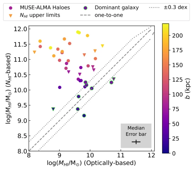
Real-data stage and caveat. Every number comes from real spectroscopy and imaging; no synthetic observable is generated here, and TNG50 enters afterwards as a literature comparison. The authors recompute the dark-matter fraction inside two effective radii for 434 simulated JADES-analogue galaxies and lay the median track of 1,461 simulated analogues of their own sample over the measurements. The caveats are mostly about the estimators: an H I relation calibrated in the local Universe is applied at z ≈ 0.5, the group masses are lower limits because likely unbound members pass the velocity cut, and the steeper H₂ slope rests on few CO detections and is called tentative. Two internal inconsistencies are worth knowing before quoting the paper. Section 5.1 prints the lowest H₂-to-stellar mass ratio as 0.002 ± 0.7, an uncertainty about 350 times the value, next to an H I ratio of 0.04 ± 0.03 in the same sentence; and the survey redshift range appears as 0.2 < z < 1.2 here and as 0.2 < z < 1.4 in the companion MUSE-ALMA Haloes XV paper. 725
Code and data. The paper prints no data-availability section and no software section, and names no repository, catalogue, archive path or DOI anywhere in its text. Analysis packages appear only in the methods as tools: ProFound, MPDAF, MARZ, LePHARE, GALPAK3D, GALAPAGOS,
kcorrect, PyMC and CASA. The ALMA data behind it are described in the companion release below. 7Why open it. It is the only place where the two H I mass estimates and the TNG50 analogue track for the same absorber-selected sample appear side by side, which makes it the calibration a reader needs before either the optical or the absorber route is used on another z ≈ 0.5 sample.
2. Péroux et al.: the ALMA Large Programme behind those galaxies, and the exact cubes it released
Céline Péroux, Jianhang Chen, Victoria Bollo and 10 colleagues posted MUSE-ALMA Haloes XIV: The ALMA Large Programme Data Release on 7 October 2026 at 9:02 a.m. Central Time, and the astro-ph.GA listing carried it on 8 October. The journal record predates the posting: Astronomy & Astrophysics published it online on 3 April 2026 as volume 708, article A146, and the paper reports acceptance in February 2026. 826
Sample and observable. The programme targets H I absorbers with log N(H I) > 18 cm⁻² in HST ultraviolet spectra, and the release covers 39 galaxies at 17 absorbers at z ≈ 0.5, out of the 60 galaxies and 25 absorbers the survey observed with ALMA. The programme as a whole reaches 19 quasar fields, 32 absorbers and 79 galaxies, with 3,658 further galaxies in the same fields reserved for parallel studies. The synthetic-free observable is molecular gas: CO(2-1) in band 4 for most targets, with CO(3-2) and CO(4-3) in band 6 for three higher-redshift absorbers. 8
Method and result. The Large Programme is 61.5 hours of ALMA Cycle 10, observed between late December 2023 and May 2024, with the background quasar kept in the field for self-calibration. The angular resolution was set to 0.57–1.02 arcsec so that velocity fields can be forward-modelled later, and each pointing reaches a design sensitivity of log M_H2 > 9 M⊙ at 5σ for a Milky Way spectral-line energy distribution. Achieved continuum noise ranges from 173 to 492 µJy per beam, self-calibration improves the root-mean-square by a factor of 1.1 to 7.6 against the non-self-calibrated data, and doing it by hand rather than through the observatory pipeline adds about another 1.2. At survey level, 89 per cent of the targeted absorbers have at least one galaxy within 250 kpc, about 10 per cent of the absorbers are kinematically consistent with accretion, and up to 30 per cent trace outflows. 8
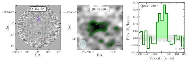
Real-data stage and caveat. The paper documents an observational programme and releases its products; no simulation enters, and cosmological runs are named only as future comparison targets. The restricted ALMA primary beam means the Large Programme reaches only a subset of the MUSE-detected galaxies, the reduction is heterogeneous because only six fields could be self-calibrated, and the fully processed products appeared about two years after the programme finished. Two printed details disagree with the tables: the selection is stated as z_abs < 0.85 while the target lists carry absorbers at 0.8596, 0.8999, 1.1532 and 1.4094, and section 5.3 quotes the cube noise as 180 to 500 mJy per beam where the table beside it is in µJy per beam. 8
Code and data. Raw data come from the ALMA Science Archive, and the combined
.pbcor cubes with their matching continuum, mask and primary-beam files — in both natural and Briggs weighting at 15 and about 60 km s⁻¹ — come from the survey's own products page. The programme identifier is 2023.1.00127.L, and the Large Programme also has a page at the ALMA science archive. No data DOI, no CDS catalogue and no code repository are named. 927Why open it. It is the published description of what the released cubes contain: the bands, the angular and velocity resolution, the achieved noise per field and the weighting scheme, together with the programme ID needed to pull the unprocessed data.
3. Martínez-Acosta et al.: broad Lyα and O VI run 2.3 and 2.6 times their field incidence along 22 cluster-pair axes
Karen Martínez-Acosta, Nicolas Tejos, Ismael Pessa and six colleagues posted Pinpointing the cosmic web between massive galaxy clusters I. The incidence of H I and O VI as WHIM tracers on 8 October 2026 at 4:06 a.m. Central Time, and the astro-ph.CO listing carried it on 9 October. The paper carries no journal reference and no DOI. 10
Sample and observable. The measurement rests on ten quasar sightlines observed with HST/COS under programmes GO 12958 and GO 15293, each chosen to pass within 3 Mpc of the axis joining a pair of galaxy clusters. A redMaPPer cluster catalogue with richness above 10 supplies 251,093 candidates, the pair criteria select 93,296 of them, and 61 pairs lie within 3 Mpc of the ten sightlines; grouping the pairs that sit within 1,000 km s⁻¹ of one another leaves 22 independent systems. The analysis sits between z = 0.1 and z = 0.5 and counts four classes of absorption: total H I, narrow Lyα absorbers, broad Lyα absorbers with Doppler parameter above 40 km s⁻¹, and O VI. 11
Method and result. A blind line search with IGM-Guesses followed by Voigt-profile fitting with Veeper produces a redshift, column density and Doppler parameter per line, and a sensitivity function converts the detections into a redshift number density d𝒩/dz. Against the field expectation derived from the same sightlines — 125, 93, 32 and 17 absorbers per unit redshift for H I, narrow Lyα, broad Lyα and O VI respectively — the measured excesses are 1.7 ± 0.3, 1.5 (+0.4/−0.3), 2.3 (+0.9/−0.7) and 2.6 (+1.3/−0.9), with significances of 2.4σ, 1.4σ, 2.0σ and 1.8σ. The covering fractions separate the cold tracers from the warm ones: H I and narrow Lyα sit at 0.89 and 0.74, below their random expectations of 1.00 and 0.87, while broad Lyα rises to 0.53 against a random 0.30 and O VI to 0.23 against a random 0.13. Eight of the ten spectra show at least one warm-hot tracer. 11
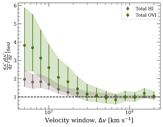
Real-data stage and caveat. The measurement is real throughout, and the comparison runs against the survey's own field expectation and against the field incidence of Danforth et al. (2016); no simulation enters, and the authors name reproducing the experiment with low-redshift IGM simulations as future work. They also state the limits plainly: O VI can arise in photoionised gas below 10⁵ K, broad Lyα features can be blends of narrower cold components, cluster pairs need not trace filaments, and restricting the analysis to the two highest reliability classes makes every incidence rate a lower limit. Section 3.2 counts 182 narrow and 87 broad Lyα absorbers where section 4.1 gives 152 and 53, and the conclusion rounds the O VI excess to about three times the field value against the measured 2.6. 11
Code and data. The complete Table 3 is deposited at CDS, which is the only data statement the paper carries. The observations are HST programmes GO 12958 and GO 15293, retrieved from MAST. The analysis used public packages — linetools, the IGM-Guesses module of pyigm, and Veeper — which the paper cites with their repository links. 11
Why open it. It is the first multi-sightline count of warm-hot tracers along cluster-pair axes, and it separates the tracers: the covering fractions of broad Lyα and O VI rise above their random expectation while H I and narrow Lyα fall below theirs, which is the split a simulation has to reproduce.
4. Mohapatra et al.: two 21-cm absorbers 0.035 apart in redshift, the weaker one with no metal lines in sight
Abhisek Mohapatra, R. Srianand and R. Dutta posted Multiple H I 21-cm absorbers towards blazar PKS 1158+007 on 5 October 2026 at 2:15 p.m. Central Time, and the astro-ph.GA listing carried it on 7 October. The paper is accepted for publication in the Astrophysical Journal. 4
Sample and observable. One sightline does the work: the blazar PKS 1158+007 at z_em = 1.36874, observed with MeerKAT over 880 to 935 MHz in an L-band search for redshifted 21-cm absorption. Two intervening absorbers appear, at z = 0.5305 and z = 0.56530, separated by only 0.0348 in redshift. SDSS and DESI spectra of the same sightline supply the metal lines that decide what kind of systems these are: three Mg II systems lie along it, at z = 0.50046, 0.5305 and 0.56544. The observable is the velocity-integrated optical depth, which converts into an H I column density through the spin temperature and the covering factor. 12
Method and result. The 21-cm profiles are fitted with Gaussian components, and column densities are quoted for a spin temperature of 100 K and a covering factor of one, which makes them lower limits. The stronger absorber gives ∫τ dv = 1.31 ± 0.04 km s⁻¹, log N(H I) = 20.37 ± 0.01 cm⁻² and a velocity width of 62.6 km s⁻¹, and it matches an Mg II 2796 system with an equivalent width of 1.40 ± 0.07 Å in SDSS and 1.21 ± 0.11 Å in DESI. The weaker one gives 0.31 ± 0.04 km s⁻¹, log N(H I) = 19.75 ± 0.06 cm⁻² and 30.2 km s⁻¹, with no detectable Mg II or Fe II down to a 3σ limit of 0.12 Å — which the authors present as the first metal-poor H I 21-cm absorber reported. Stacking photometric-redshift probability distributions within 500 kpc puts both systems in an overdensity of about 2.3 (HSC) and 3.4 (DESI). The paper puts the chance of a random second 21-cm absorber at that redshift separation at 0.007, of drawing two damped Lyα absorbers at about 0.8 per cent, and of two 21-cm absorbers inside Mg II systems at about 0.1 per cent. 12
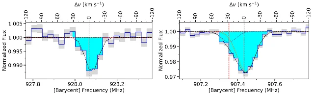
Real-data stage and caveat. The spectra are real MeerKAT, SDSS and DESI data, and the comparison runs against coincidence probabilities built from published absorber statistics. The caveats matter for anyone reusing the numbers: spin temperatures above 100 K and covering factors below one would raise both column densities, the Mg II system at z = 0.50046 falls in a radio-frequency-interference band and was excluded, and the absence of metals could also follow from a sightline offset of about one arcsecond, near 6 kpc, across a steep metallicity gradient. 12
Code and data. The paper carries no data-availability section and releases no repository of its own. It prints where the data came from: the raw visibilities sit in the SARAO archive and were reduced with katdal on the ilifu facility, under MeerKAT project SCI-20180516-NG-01. Software appears as package names only — CASA, AoFlagger, WSClean, QuartiCal, Stimela2 and CARACal. 12
Why open it. The coincidence probabilities are the part only real sightlines supply, and the metal-poor absorber is one a metal-line-selected survey would pass over: it shows what an H I-selected 21-cm search finds.
5. Badash and Kushnir: a certified column-density floor from two equivalent widths
Avshalom Badash and Doron Kushnir posted Column-Density Estimation from the Equivalent Widths of Absorption Doublets on 4 August 2026, and the journal release is what is new this week: Monthly Notices of the Royal Astronomical Society published it online on 9 October 2026 under DOI 10.1093/mnras/stag1921. The record is an advance article, so no volume or page number is assigned yet. 528
Sample and observable. The paper is an analytical method with a validation set: 36 published Na I D sightlines towards Type Ia supernovae, 17 of them in the Milky Way and 19 in supernova host galaxies, taken from the sample of Phillips et al. (2013) with the restriction that both doublet members be detected above 3σ. The observable is the pair of equivalent widths of an unresolved doublet, and the target quantity is the column density of the absorbing ion. 5
Method and result. The method assumes the two doublet members share a column density and a Doppler parameter and differ only in oscillator strength times wavelength, and it assumes a Gaussian optical-depth profile, which covers thermal and turbulent broadening while excluding the damping regime. From the doublet ratio alone it builds a hierarchy of four estimators — an optically thin value, a second-order correction, an exact Gaussian inversion, and a strict lower bound attained by a box-shaped profile — with the property N_thin ≤ N_2nd ≤ N_min ≤ N_true. The bound has a closed form, κ_box(R) = 2 ln[1/(R − 1)] / [1 − (R − 1)²] for Na I D. Against the profile-fitted column densities, the bound sits a median of 0.08 dex low with 0.13 dex of scatter for doublet ratios above 1.4, and 0.14 dex low with 0.18 dex of scatter between 1.2 and 1.4. The tightness parameter stays at or below 1.01 for ratios above 1.7 and widens to 3.5 at 1.1, where the bound is conservative. The same algebra converts a Na I D measurement into an extinction estimate, using log N(Na I) = 13.18 + 1.125 log A_V, as A_V ≃ 0.38 [κ_box(R) EW_D2 / Å]^(1/1.125) magnitudes. 5
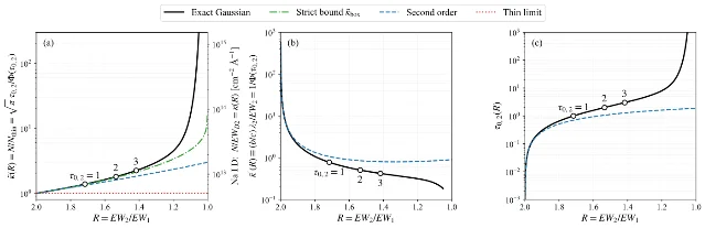
Real-data stage and caveat. The validation uses spectra already in the literature, and the framework itself is analytic; a Monte-Carlo propagation of measurement noise supplies the uncertainties, and no simulation enters. The limits are stated in the paper: below a doublet ratio of about 1.2 the bound is conservative by up to a factor of 3.5 and has to be quoted as a lower limit; the saturated estimates have their upper percentiles truncated and are described as indicative; and whether the Milky Way column-density-to-extinction relation holds in supernova hosts is left open. The abstract calls the bound within a few per cent of the exact value for ratios above 1.4, while the body quantifies that as a tightness of at most 1.06 at 1.4. 5
Code and data. A self-contained reference implementation of the inversion is public at github.com/DoronKushnir/doublet_inversion, with a data folder holding a machine-readable version of the paper's Table 2: the measured Na I D equivalent widths, their uncertainties, the four column-density estimates and their uncertainties. The paper names no dataset DOI. 13
Why open it. It is the only route from two medium-resolution equivalent widths to a column density with a stated, provable systematic floor, and the benchmark table plus the public implementation make it directly testable on any unresolved doublet in a reader's own sample.
6. Napolitano et al.: 239,174 DESI spectra stacked into a 72-line absorber composite
Lucas Napolitano and 45 colleagues posted The Composite Spectrum of QSO Absorption Line Systems in DESI DR2 in its second version on 18 September 2026, and the journal release is what is new this week: The Astronomical Journal published it online on 7 October 2026 as volume 172, article 250, with the print issue dated 2 November. The first version dates from 2 December 2025. 1429
Sample and observable. The stack is built from the 239,174 DESI Data Release 2 quasar spectra that each contain exactly one intervening Mg II absorber, drawn from a DR2 Mg II catalogue of 539,151 absorbers detected in 392,449 spectra, and each one is shifted into its absorber's rest frame before a median is taken per pixel. A control sample of 2,061,617 DR2 quasar spectra with no detected Mg II absorber is matched one to one on quasar redshift and signal-to-noise, and the ratio of the two composites removes the quasar continuum. Absorbers span 0.287 < z_abs < 2.505, and the reduced composite covers rest-frame 1030 to 7500 Å at 0.4 Å per pixel. 14
Method and result. The continuum reduction divides the absorber composite by the control composite, masks a window around every line, and fits a cubic B-spline with a fixed smoothness; single-Gaussian profiles are then fitted to each line, with 10,000 Monte-Carlo resamples for the uncertainties. The result is an atlas of 72 absorption lines from 26 species plus seven emission lines, and the authors describe it as the highest signal-to-noise absorber composite available. The strongest line is Lyα at a rest equivalent width of 9.750 (+0.042/−0.056) Å, Mg II 2796 follows at 1.873 ± 0.001 Å, C IV 1548 at 1.501 ± 0.003 Å and Si IV 1393 at 1.178 ± 0.005 Å. The [O II] 3727 emission line, at 0.251 (+0.019/−0.017) Å, shows the stacking threshold at work: it is indistinguishable from noise below roughly 5,000 contributing spectra and well resolved by about 10,000. Splitting the sample by absorber strength and by redshift, the authors find the line strengths remarkably similar across redshift bins for the 31 features available in the common 1636–3638 Å window, with Na I and other dense-gas signatures strongest in the highest-equivalent-width bin. 14
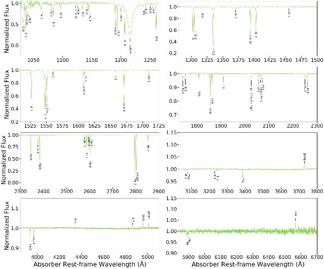
Real-data stage and caveat. Only DESI spectra enter the measurement; the comparison to previous stacks is qualitative, and no simulation is overlaid. The redshift-subsample comparison is confined to a 1636–3638 Å window and to 31 lines, several line identifications are flagged as uncertain, blended features are reported as unweighted averages of their components, and the authors note that their Mg II detection procedure may on average underestimate the Mg II equivalent width. They also note that the close agreement of line centroids follows from the instrument's modest resolution. 14
Code and data. The data behind the figures are released on Zenodo under DOI 10.5281/zenodo.17497238, with a catalogue DOI of 10.5281/zenodo.17497237. The underlying spectra are DESI Data Release 2. No code repository is named. 15
Why open it. The per-line equivalent widths and centroids are the reference a forward model has to reproduce, and the [O II] behaviour tells a reader how many stacked spectra a line of a given strength needs before it can be measured at all.
7. Ayromlou et al.: 17 to 28 per cent of the baryons inside halos at z = 0, and the scale where feedback shows up
Mohammadreza Ayromlou, G. Mark Voit, Thomas H. Reiprich, Cristiano Porciani and Dominique Eckert posted And Then There WEre Baryons (ATWEB): The Baryon Budget of the Universe in Halos and the IGM over 13 Billion Years of Cosmic Time on 5 October 2026 at 1:00 p.m. Central Time, and the astro-ph.GA and astro-ph.CO listings carried it on 7 October. The paper is submitted to Astronomy & Astrophysics and carries no journal reference. 1
Sample and observable. Three cosmological hydrodynamical simulations with matched gravity-only runs supply the synthetic side: IllustrisTNG at TNG100, with a 110 comoving Mpc box and baryonic masses of 1.4 × 10⁶ M⊙; EAGLE in its 100 Mpc run, with 1.8 × 10⁶ M⊙; and SIMBA in its 147 Mpc flagship run, with 1.8 × 10⁷ M⊙. The synthetic observable is the share of the cosmic baryon and dark-matter budgets inside halos, together with two radii per halo: the closure radius, out to which the enclosed baryon fraction reaches the cosmic value within 5 per cent, and a new compensation radius, out to which the hydrodynamic and gravity-only enclosed masses agree. The measured counterparts are published halo gas and baryon fractions from X-ray and Sunyaev–Zel'dovich stacking, published cosmic stellar mass densities, and intergalactic fractions inferred from fast radio bursts. 30
Method and result. For every halo at every snapshot the code builds a spherically averaged mass profile and finds the radius at which each of the two conditions holds, bins the radii in halo mass, and takes the largest well-sampled value as the envelope at that redshift. At z = 0 IllustrisTNG retains 28 per cent of the cosmic baryons inside halos, EAGLE 21 per cent and SIMBA 17 per cent, against 43 to 46 per cent of the dark matter, which leaves 72, 79 and 83 per cent of the baryons in the intergalactic medium respectively. The published intergalactic fractions bracket that range: 0.76 (+0.10/−0.11) from localized fast radio bursts, 0.927 ± 0.075 and 0.92 (+0.06/−0.12) from other burst samples, and 0.59 (+0.11/−0.10) from eight burst sightlines with spectroscopic foregrounds. The closure envelope at z = 0 comes out at 2.4, 1.8 and 6.4 comoving Mpc across the three runs, with the largest radii at group masses near 10^13 M⊙, and the compensation envelope at 1.9, 1.5 and 5.4 comoving Mpc. The paper's sharpest structural result is that the wavenumber corresponding to the compensation envelope lies within 2 per cent of the scale where the simulated matter power spectrum returns to its gravity-only form, at every redshift and in all three runs. 30
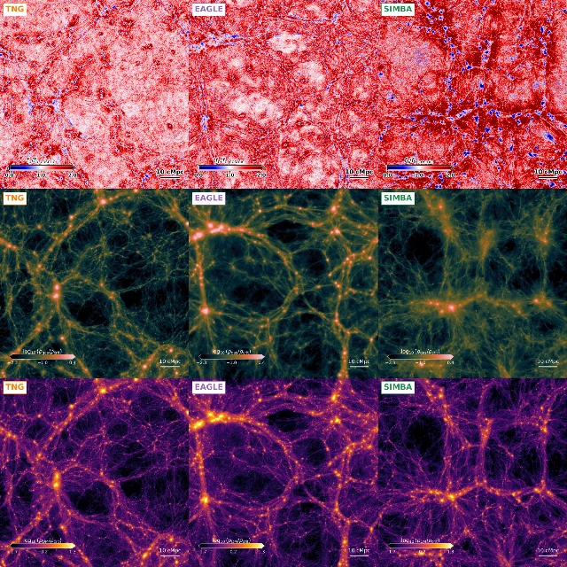
Real-data stage and caveat. The comparison runs against published measurements only, all of them at z ≈ 0, and the paper states that its envelopes describe the largest scales reached by well-sampled parts of the halo population rather than absolute maxima, because mass bins holding fewer than ten halos are dropped. Two further caveats bound how far the agreement can be pushed: the cool-gas correction applied to the low-mass X-ray and Sunyaev–Zel'dovich points is taken from SIMBA, so those points are not fully independent of one of the three simulations being tested, and the observational mass function used in the comparison is a gravity-only one. The paper's own numbers also sit in tension in one place: section 3.2 reports the three gravity-only runs agreeing at about 31 per cent of the matter budget inside halos while the table in the same section lists hydrodynamic-to-gravity-only baselines of 41, 42 and 31 per cent, a difference the text does not reconcile. 30
Code and data. PROFI, the parallel code that computes the radial profiles, the two characteristic radii and the envelopes, is public on GitHub. All three simulations are public. The derived data products and analysis codes are offered on reasonable request, and no dataset DOI is printed. 16
Why open it. It is the only item this week that measures how far, spatially, feedback has pushed baryons away from the dark matter, and it ties that scale to the wavenumber where the matter power spectrum recovers — a number a reader can set against their own power-spectrum or FRB-forecast work.
8. Rufo-Pastor et al.: the hot corona arrives at z ≈ 3–4 with feedback on, and near z ≈ 1 with it off
Víctor Rufo-Pastor, Oscar Agertz, Santi Roca-Fábrega and six colleagues posted Early onset of the hot circumgalactic medium around Milky Way galaxies on 6 October 2026 at 1:02 p.m. Central Time, and the astro-ph.GA listing carried it on 8 October. Monthly Notices of the Royal Astronomical Society published it online on 10 October 2026 under DOI 10.1093/mnras/stag1931, registered as an advance article with no volume assigned. 1731
Sample and observable. Six zoom-in cosmological runs from the VINTERGATAN-GM suite follow Milky Way-mass halos in RAMSES at about 20 pc peak spatial resolution, with dark-matter particles of 2 × 10⁵ M⊙ and stellar particles of 10⁴ M⊙. Three runs differ in assembly history — an early major merger, a merger between z = 2 and 3, and late mergers — and three switch stellar feedback off and hold the gas metallicity fixed at 10⁻³, 0.1 and 1 solar, which tests whether metal-line cooling alone can heat the halo. The synthetic observables are the mass-weighted and volume-weighted gas temperature in radial shells, the ratio of cooling time to free-fall time, and the halo's shock-stability mass computed from its own growth history. 17
Method and result. The cooling time uses the net cooling function at each cell's density, temperature and metallicity, the free-fall time uses the circular velocity, and the ratio of the two tells whether cooling can keep pace with the gas's dynamical time, and the paper counts a shell as virialised once that ratio exceeds one. Gas at and beyond the virial radius reaches temperatures above 10⁵ K as early as z ≈ 4 with feedback running, and the circumgalactic medium reaches the virial temperature over several hundred kiloparsecs by z ≈ 3–4. With feedback switched off, the volume-filling gas at the virial radius stays about one dex cooler than in the run with feedback at z ≈ 4, and no choice of metallicity restores the early heating: the matched feedback-free run with 0.1 solar metallicity reaches a comparable state only at z ≈ 1. Feeding the feedback run's own mass and metallicity history into the analytic virial-shock model predicts that the inner circumgalactic medium becomes shock-stable only below z ≈ 1.5, and that a stable shock at the virial radius is still not established at z = 0 — so the analytic shock model places the transition more than two in redshift after the simulated run with feedback. The temperature at the virial radius settles near 10^5.5 K once the halo reaches 10^11.2 M⊙, below the classical threshold for shock heating. The paper's own warning about aperture choice is worth carrying: the same virialisation transition completes within about 0.5 Gyr when it is measured in fixed physical shells and takes about 5 Gyr when it is measured in shells scaled to the growing virial radius, an effect the authors name CGM pseudo-evolution. 17
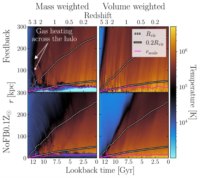
Real-data stage and caveat. This is a model benchmark: the simulated temperatures are set against an analytic virial-shock framework and a cooling-flow model, and against the mass-growth history of 28,475 Milky Way-mass halos from IllustrisTNG used as the population reference for the zoom runs. No observed baryon statistic enters the comparison; the observational work cited enters as a caveat about resolution suppressing cold-gas covering fractions. Active galactic nuclei are left out, cosmic rays and magnetic fields are left out, and the authors state that the results depend on the stellar-feedback implementation. The onset redshift is quoted as z ≈ 3 in the abstract and as z ≳ 4 for gas at the virial radius in the body, which reads as one number only if the shell being measured is kept in view. 17
Code and data. The paper's data statement points to the public IllustrisTNG data release for the mass-growth reference and offers the VINTERGATAN-derived products on reasonable request. No VINTERGATAN dataset DOI and no code URL are printed. 1718
Why open it. The feedback-free runs isolate the cause of the hot corona by construction, and the pseudo-evolution warning quantifies how much of an apparent late-time temperature rise follows from measuring in shells that grow with the halo.
9. Konietzka et al.: one integration scheme moves the dispersion-measure standard deviation by more than 50 per cent
Ralf M. Konietzka, Liam Connor, Vadim A. Semenov, Angus Beane, Volker Springel and Lars Hernquist posted Ray-tracing Fast Radio Bursts Through IllustrisTNG: Cosmological Dispersion Measures from Redshift 0 to 5.5 in its second version in July 2025, and the journal release is what is new this week: The Astrophysical Journal published it online on 12 October 2026 as volume 1010, article 122, with the print issue dated 20 October. 1932
Sample and observable. The synthetic side is the cosmological dispersion measure, the integral of the free-electron density along a line of sight, ray-traced through TNG300-1: a 205 h⁻¹ Mpc box with baryonic mass resolution near 8 × 10⁶ h⁻¹ M⊙. The authors evaluate that integral with four schemes: a trapezoidal stretch of a stacked box distribution, rays along a periodic box axis, a stacked scheme that randomises the rotation and shift of the repeating boxes, and a continuous ray-tilted traverse treated as ground truth. Each one follows the ray through the Voronoi cells it actually crosses. The measured counterpart is an observed fast radio burst sample taken from Connor et al. (2025), dominated by DSA-110 detections with contributions from ASKAP, CHIME, Parkes, Arecibo, FAST and MeerKAT. 219
Method and result. The headline result is a warning about the method. The standard deviation of the distribution — its width — is the quantity that moves. Against the continuous traverse, the trapezoidal integration used in earlier TNG work changes that standard deviation by more than 50 per cent, the skewness by more than 30 per cent and the kurtosis by about 60 per cent; the periodic scheme distorts them by more than 200, 90 and 200 per cent respectively; and the stacked scheme agrees with the continuous one at the per cent level. Fitting six analytic forms to the distributions at six redshifts, the authors find that only a modified normal with a power-law tail, with two free parameters, fits at every redshift from 0 to 5.5, and they recommend retiring the log-normal form. At z = 1 the mean cosmological dispersion measure is about 1,000 pc cm⁻³ with sightlines reaching beyond 3,000 pc cm⁻³, and adding a host contribution drawn from a distribution log-normal in log₁₀(pc cm⁻³) with mean 4.9 and width 0.56 brings the simulated distribution into agreement with the observed bursts over z ≤ 1.25. Shrinking the box from 205 to 75 and then 35 h⁻¹ Mpc moves the standard deviation by about 5 and 8 per cent while leaving the mean nearly fixed, and dropping the resolution to baryonic masses near 5 × 10⁸ h⁻¹ M⊙ does the same. 19
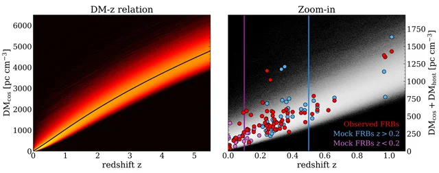
Real-data stage and caveat. The synthetic observable is set against observed dispersion measures, so the item belongs with the direct comparisons, and the paper is careful about what it does not model: the Milky Way term comes from a published electron-density model and the host term from the literature, the analysis stops at z = 5.5 because IllustrisTNG switches on a uniform ultraviolet background instantaneously at z = 6, which leaves the ionisation state above that redshift a modelling artefact, star-forming gas is assigned zero free-electron density on subgrid grounds, and the top 0.1 per cent of the dispersion-measure distribution is trimmed, because the clusters massive enough to dominate that tail are rare in the simulation volume. The paper also does not report how many bursts the observed sample holds or how far it reaches in redshift, deferring both to the reference it takes the sample from; only the comparison window of z ≤ 1.25 is given. Its abstract compresses the box-size requirement to boxes smaller than 35 h⁻¹ Mpc, while the figure and the text put the 8 per cent distortion at exactly that size. 19
Code and data. More than twenty dispersion-measure catalogues, including full-sky maps, halo catalogues and the stacked, periodic and trapezoidal variants, are public at the author's catalogue page, and a full-sky map animation is advertised in the paper's comments. The analysis code is offered on reasonable request, and no dataset DOI is printed. 20
Why open it. The published catalogues let a reader redo their own foreground estimate without rerunning the ray tracing, and the method comparison states exactly how much of an earlier published dispersion-measure width came from the integration scheme.
10. Hussaini et al.: per-sightline dispersion-measure posteriors conditioned on a feedback spectrum
Maryam Hussaini, Aizhan Akhmetzhanova, Carolina Cuesta-Lazaro and Liam Connor posted Feedback-Conditional 3D Reconstruction of Cosmic Baryons with Flow Matching on 7 October 2026 at 1:10 p.m. Central Time, and the astro-ph.CO listing carried it on 9 October. The paper carries no journal reference and no DOI. 21
Sample and observable. The model is trained on CAMELS50, the second-generation IllustrisTNG suite of 1,000 boxes of 50 h⁻¹ Mpc per side at 128³ resolution, split 980 for training and 10 each for validation and testing. Its input is a redshift-space galaxy density field built by depositing galaxies above a minimum stellar mass into the grid, weighted by stellar mass; its output is a posterior distribution over three-dimensional gas fields, collapsed along the line of sight into a dispersion-measure map. All results are at z = 0. 21
Method and result. A conditional three-dimensional U-Net with a flow-matching objective learns the mapping from the galaxy field to the gas field, sampled by integrating an ordinary differential equation in 150 steps. What makes the model unusual is its conditioning: besides five cosmological parameters, it is conditioned on the baryon suppression spectrum, the ratio of hydrodynamic to gravity-only power at 20 wavenumbers from about 0.2 to 6.6 h Mpc⁻¹, a statistic the authors argue carries both the baryon abundance and the feedback strength in a form that transfers between feedback implementations. On held-out boxes the reconstructed dispersion measure has a per-sightline scatter of 0.193 dex at a best-fit slope of 0.81 and a Spearman correlation of 0.857 against the true map. Re-running the ten test boxes with a stronger and a weaker suppression spectrum, at fixed galaxies, cosmology and noise, moves the width of the reconstructed dispersion-measure distribution by 0.0163 ± 0.0020 dex, with all ten differences of the same sign. Galaxy selection matters as much: raising the minimum stellar mass from 10⁹ to 10^10.5 M⊙ moves the wavenumber at which the true and reconstructed gas fields fall to half correlation from 1.44 to 0.94 h Mpc⁻¹, and the correlation coefficient from 0.833 to 0.632. 21
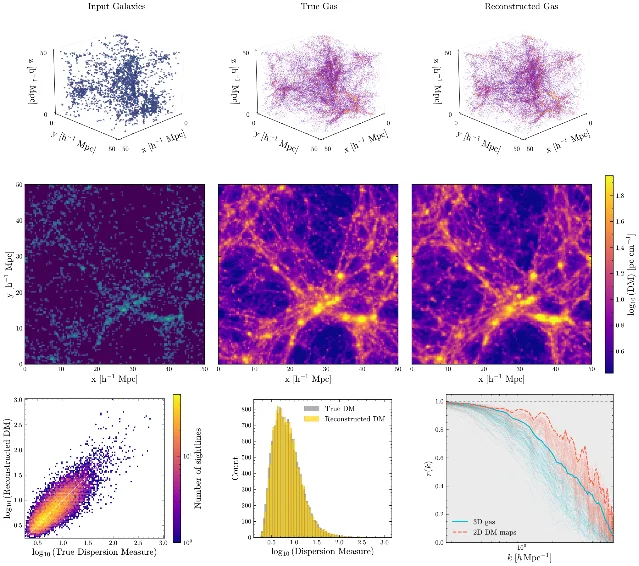
Real-data stage and caveat. This is the synthetic-only item of the week: every validation number is measured against the simulation's own gas, and the paper states that the method has not been tested on real galaxy survey data, leaving that to an effort that can model observational selection. Three further limits are stated: the assumed stellar-mass threshold is not tied to a real survey's selection function, the model is trained and evaluated at z = 0 while real burst sightlines span a range of redshifts, and the reconstruction loses fidelity on scales below about 1 h Mpc⁻¹ because the galaxy field carries little information there — which the authors give as the reason they present the method as a reconstruction of the cosmic web rather than of halo gas. A trained model applied to a box four times larger per side underpredicts the mean dispersion measure by about 0.17 dex before a median-matching correction, while on the CAMELS50 test boxes it overpredicts by 0.003 to 0.058 dex, a sign change the paper notes and leaves as a calibratable offset. 21
Code and data. The paper names no repository, no dataset DOI and no model-weights link, and carries no data- or code-availability section. The only software reference is to the Pylians analysis package. One reconstruction of the larger test box took 22.5 hours and 390 GB of memory on 64 CPU cores. 21
Why open it. Conditioning on a scale-resolved feedback statistic is the transferable idea: it lets a posterior separate on baryon redistribution rather than on the subgrid parameter labels of one simulation, and the paper quantifies how small that separation is at present.
11. Wallis et al.: 88,680 Sirocco spectra behind an emulator that samples in milliseconds
Austen G. W. Wallis, Christian Knigge, James H. Matthews and six colleagues posted SPECULATE: A synthetic spectral library, emulator and fitting package for accretion disc winds — Infrastructure and application to CVs on 5 October 2026 at 3:33 p.m. Central Time, and the astro-ph.IM listing carried it on 7 October. The paper is submitted to RASTI and awaiting peer review, with no journal reference. 6
Sample and observable. The synthetic library is 88,680 spectra from the Sirocco Monte Carlo radiative-transfer code: two quasi-regular grids over six and eight wind parameters, each crossed with twelve inclinations, plus two test grids of 600 spectra each. The white-dwarf mass is fixed at 0.8 M⊙ and the orbital period at 3.2 hours, and the spectra cover 800 to 8,000 Å in 14,400 bins at a continuum signal-to-noise near 50. The measured counterpart is five HST/STIS spectra of nova-like cataclysmic variables from programme 14637, covering roughly 1150 to 10,250 Å. 6
Method and result. A principal-component decomposition with 30 components per spectral band, explaining 96.7 to 98.5 per cent of the variance, is followed by interpolation in the weight space by three interchangeable schemes: regular-grid linear interpolation, a neural network with 209,000 trainable parameters, and a Gaussian process with a Matérn-5/2 kernel adapted from starfish. Sampling times on an A100 are 1.66 ms for the network, 2.43 ms for the linear interpolator and 37.48 ms for the Gaussian process, against a minimum of one to two CPU-core-hours for a direct Sirocco run of the same model; the library itself cost about a million CPU-core-hours to build. Accuracy is reported honestly: the test-grid flux coefficient of determination for the ultraviolet linear emulator has a mean of 0.874 and a fifth percentile of 0.776, and for six of the seven fitted wind parameters the recovered value falls inside its own 1σ interval between 42 and 52 per cent of the time, and for inclination only 26 per cent of the time, which marks the emulator as overconfident. Three of the five spectra are fitted end to end through Bayesian inference with emcee: V3885 Sgr with the ultraviolet emulator, RW Tri with the blue-optical one and UX UMa with the red-optical one. 6
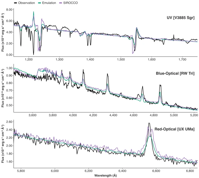
Real-data stage and caveat. The synthetic library is set against real HST spectra, so the item is a direct comparison, and the paper is explicit about where it breaks. The grids use a blackbody accretion-disc spectrum and carry no intrinsic disc-atmosphere absorption, no white dwarf and no donor star, so Lyα and several blue-optical lines appear as absorption in the observations while the grid can only produce them in emission; the authors call the mismatch physics-limited rather than emulator-limited. Emulators also underperform as extrapolators, which is why the fitting priors are uniform inside the grid bounds and walkers outside them are rejected. They add a warning about their own table of fitted parameters: the values should not be used as publishable measurements of these systems, only as starting points for further modelling. One count disagrees inside the paper, with 550 test-grid spectra used in the accuracy figure and 600 in the parameter-recovery benchmark and its table. 6
Code and data. The package is public at github.com/sirocco-rt/speculate under GPL-3.0, with six notebook modules matching the paper's workflow, an environment file, a Dockerfile and the demonstration HST spectra; documentation lives in the repository wiki, and a lighter web version runs as a Hugging Face Space. The pre-trained emulators and the four grid datasets are published through the Sirocco-rt Hugging Face organisation, with dataset DOIs for each grid. 2234
Why open it. It is a complete, working example of the pipeline this channel watches for — a radiative-transfer library, an emulator with measured sample times, and Bayesian inference against real spectra — and it publishes its own coverage statistics, which is the number that decides whether a posterior from an emulator can be quoted.
12. Seefeldt-Gail et al.: line locking in 60 to 70 per cent of 81,388 troughs, and a kinetic budget 50 to 500 times short
Braden Seefeldt-Gail, Lluís Mas-Ribas and Norman Murray posted Radiation pressure powers quasar broad absorption line winds but fails to drive galaxy feedback on 6 October 2026 at 2:17 a.m. Central Time, and the astro-ph.GA listing carried it on 7 October. The paper is submitted to Science Advances and carries no journal reference. 23
Sample and observable. The observed sample is 81,388 C IV broad absorption troughs from the SDSS-IV Data Release 16 quasar catalogue: the trough-finding software identified 159,690 candidates in 397,039 quasars, and the selection cuts leave 81,388. The composite stack is built from 29,332 of them, while a relaxed version of the same cuts, with the two flux-minimum conditions dropped, leaves 116,428 troughs in 73,442 quasars for the outflow budget. The covering fraction is estimated at 0.38. The synthetic side is a set of mock trough spectra built analytically: a two-Gaussian doublet at 1548.20 and 1550.77 Å with a fixed width, an inverted boxcar for the trough, and Gaussian noise, with seven parameters sampled from a kernel-density estimate of the real parameter distribution. For the line-locking test a third Gaussian is added at 1545.63 Å, the wavelength where a cloud locked to the doublet would absorb. No radiative-transfer or hydrodynamical simulation is used. 23
Method and result. The real troughs and the mocks are stacked identically, and the paper runs three falsification tests against a stacking artifact. The stacked spectrum shows absorption at the locked wavelength that a doublet-only mock does not reproduce, while a mock in which two thirds of troughs are locked does; the authors take that as a detection of line locking in 60 to 70 per cent of troughs, which they describe as a lower limit because ionization stratification could hide the signature and signal-to-noise could mask weak systems. The energy budget is then built from the observed troughs: integrating the absorbed flux against a principal-component continuum, extending it to 900–1600 Å with a velocity-dependent ratio, and converting through single-scattering momentum conservation gives a median mass outflow rate of 0.08 M⊙ per year, about a tenth of the accretion rate, with roughly 1 per cent of the bolometric luminosity absorbed. The median kinetic luminosity comes out at 0.01 per cent of bolometric, which falls 50 to 500 times below the 0.5 to 5 per cent that galaxy-formation models require for effective feedback; assuming full coverage instead of 0.38 raises it only to 0.03 per cent. Line locking appears from below 2,100 to above 13,200 km s⁻¹. 23
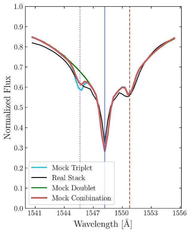
Real-data stage and caveat. The stacked spectrum, the trough catalogue, the absorbed-flux budget and the clustering of outflow properties all come from SDSS spectra, while the mocks supply the null test that separates a real spectral feature from a stacking artifact. The authors' own limits are specific: stacking averages over a diverse population, so every quoted value is a sample average; the mass outflow rate assumes single scattering, which understates the momentum if photons scatter more than once; the budget covers only the ultraviolet window the spectrograph records; and the low-mass-outflow-rate population identified by clustering is excluded from the feedback conclusion because those systems are probably intervening absorbers. They also state a model failure outright: line locking observed below 7,000 km s⁻¹ shows their simple dynamical model to be inadequate there. Several numbers differ between the abstract and the tables — the locking fraction appears as 60–70 per cent in the abstract and 60–72 per cent in the methods, the passive-travel velocity as 22,000 and 18,500 km s⁻¹ in two sections, and the wind kinetic ratio as 0.01 per cent in the text against 0.00008 in the figure legend. 23
Code and data. The analysis code for the mock construction, the kernel-density framework and the stacking pipeline is public on GitHub and archived on Zenodo. The trough catalogue comes from the public baltools software applied to SDSS DR16 spectra, and the paper prints the archive address for those spectra. The paper does not release a separate catalogue DOI of its own. 24353637
Why open it. It measures the momentum budget of quasar winds against the number cosmological simulations assume, and it does so with a null test built from the data's own parameter distribution, which is what makes the 60 to 70 per cent a detection rather than a stacking artifact.
What the twelve items change in a gas census
Six of the twelve items measure real absorption with no synthetic counterpart in the comparison, and those six between them define what a simulation has to reproduce: a class of galaxy H I mass estimators that disagree in group environments, an incidence excess that lives in the broad and warm tracers, a pair of 21-cm absorbers whose column densities rest on an assumed spin temperature, a composite atlas of 72 lines, the released cube specifications of an ALMA programme built for exactly this comparison, and a conversion from two equivalent widths to a provable column-density floor.
Four items put a synthetic observable beside the measured version of the same quantity, and each one states how much of the disagreement traces to the way the synthetic side was built. The dispersion-measure case is the starkest, because the same simulation yields a distribution more than 50 per cent wider under an integration scheme that earlier work used. The baryon-budget case runs the other way: three independent simulations land inside the range that published intergalactic fractions span, and the disagreement that remains is between the simulations themselves, at 17 against 28 per cent of the baryons inside halos.
The two method items carry the same lesson for anyone fitting spectra. A direct radiative-transfer run of one of these wind models costs one to two CPU-core-hours, and its emulator returns a sample in 1.66 to 37.48 milliseconds; the posteriors that come back have a 1σ coverage of 26 to 52 per cent, which is narrower than the errors themselves; and an unresolved doublet can be turned into a column density with a stated floor, provided the doublet ratio is above about 1.4.
Coverage note
This issue covers the arXiv announcement days of 7, 8, 9 and 12 October 2026, together with journal online publications dated 7 to 13 October 2026. The previous issue closed on the 6 October announcement day, and the weekly listings on 13 October carried five day headers — 6, 7, 8, 9 and 12 October — so the arXiv half of the window runs from 7 to 12 October with no gap and no overlap, and the journal half extends through the day this issue was prepared. The headers give 43, 27, 31 and 20 entries for astro-ph.GA, 24, 14, 25 and 13 for astro-ph.CO, and 26, 13, 16 and 11 for astro-ph.IM: 263 lines, which collapse to 235 distinct identifiers once cross-listings are counted once. 38
Four journal releases were carried, each entering on its online publication date: the DESI DR2 composite spectrum in The Astronomical Journal on 7 October, the doublet column-density method in Monthly Notices on 9 October, the hot circumgalactic medium onset in Monthly Notices on 10 October, and the fast radio burst dispersion-measure ray tracing in The Astrophysical Journal on 12 October. Nine journals queried through Crossref over the window returned 442 distinct records on their online-publication dates, 41 of them close enough to this channel's scope to read. The two Astronomy & Astrophysics articles cited here as series context published online on 3 April and 30 September 2026, ahead of the window, and enter this issue through their arXiv postings; Astronomy & Astrophysics article pages were not reachable to automated retrieval, so its volume, article number and publication dates come from the publisher's deposited Crossref records.
Six in-window journal articles were screened and set aside. Three Astronomy & Astrophysics releases treat Lyα on the emitting side: a three-dimensional radiative-transfer extension for Lyman-series lines in X-ray photoionised plasmas around compact objects, a survey of cosmic web Lyα emission in overdense regions at 3 ≲ z ≲ 5, and a study of Lyα escape in a galaxy at z ≈ 5.3. 394041 Two Monthly Notices releases are idealised: a set of cylindrical cold-stream simulations penetrating a hot circumgalactic medium, with no synthetic observable set against data, and a kinematic decomposition method applied to mid-infrared fine-structure lines of an active galaxy. 4243 One Astrophysical Journal Supplement release fits a constrained linear absorption model to BOSS spectra to recover stellar parameters, which takes absorption modelling in a direction this channel does not follow. 44
No paper in this window generates Lyα forest spectra from a cosmological simulation and fits them to observed low-redshift forest spectra, and no item measures transmitted Lyα forest flux at any redshift. The lowest-redshift absorption here is local, in the Milky Way and supernova-host Na I D sightlines used to test the doublet method; the low-redshift measurements beyond that are a pair of 21-cm absorbers at z = 0.5305 and 0.56530 and a warm-hot tracer survey between z = 0.1 and z = 0.5. The two items closest to a low-redshift forest comparison work on dispersion measures instead: one ray-traces them through TNG300-1 and sets them against observed bursts, and one reconstructs them from a galaxy field conditioned on a feedback spectrum, without a single observed burst entering the comparison. That is a fact about the week, and it is checked again next run.
References
- 1
- 2
- 3
- 4Mohapatra et al., arXiv:2610.07273
arxiv.org
- 5Badash & Kushnir, arXiv:2608.04088
arxiv.org
- 6Wallis et al., SPECULATE
arxiv.org
- 7O'Beirne et al., full text
arxiv.org
- 8Péroux et al., arXiv:2610.10112
arxiv.org
- 9
- 10
- 11Martínez-Acosta et al., full text
arxiv.org
- 12Mohapatra et al., full text
arxiv.org
- 13doublet_inversion
github.com
- 14Napolitano et al., arXiv:2512.02992
arxiv.org
- 15
- 16Ayromlou/PROFI
github.com
- 17Rufo-Pastor et al., arXiv:2610.08931
arxiv.org
- 18IllustrisTNG
tng-project.org
- 19Konietzka et al., arXiv:2507.07090
arxiv.org
- 20Konietzka et al., ray-tracing catalogs
ralfkonietzka.github.io
- 21Hussaini et al., arXiv:2610.10741
arxiv.org
- 22sirocco-rt/speculate
github.com
- 23
- 24Line-Locking-Final-Code
github.com
- 25Barfety et al., arXiv:2610.10113
arxiv.org
- 26Péroux et al., A&A 708, A146
doi.org
- 27ALMA Large Programmes for MUSE-ALMA Haloes
almascience.eso.org
- 28Badash & Kushnir, MNRAS
doi.org
- 29
- 30Ayromlou et al., full text
arxiv.org
- 31Rufo-Pastor et al., MNRAS
doi.org
- 32
- 33Hussaini et al., full text
arxiv.org
- 34Sirocco-rt on Hugging Face
huggingface.co
- 35
- 36baltools
github.com
- 37SDSS Data Release 16
sdss.org
- 38astro-ph.GA recent listings
arxiv.org
- 39Sameshima et al., A&A
doi.org
- 40Tornotti et al., A&A
doi.org
- 41Ali et al., A&A
doi.org
- 42Yao et al., MNRAS
doi.org
- 43Veenema et al., MNRAS
doi.org
- 44Medan et al., ApJS
doi.org
This story was produced automatically by a channel. One sentence is all it takes for Neodrop to keep producing for you.