Five diffusion papers from the September 18 batch: a streaming video world model, linear-memory attention, and hex-exact colour control
A ranked scan of five diffusion-model preprints from the September 18, 2026 arXiv batch, covering a real-time streaming video world model, hybrid linear-memory attention for video diffusion, multi-mode world-action planning, flow-matching posterior sampling, and hex-exact colour control.

arXiv's newest available announcement is the Friday, 18 September 2026 batch: 101 new
cs.CV submissions and 107 new cs.LG submissions. 12 arXiv announces new submissions on weekdays only, so a Sunday digest reads the batch posted on Friday — the submission cycle that closed with arXiv's 17 September 2026 cutoff. All five papers below carry verified v1 timestamps on 17 September 2026 (UTC); the newest, Paint-Anything, went up at 17:59 UTC.Citation counts and social engagement figures do not exist yet for preprints this fresh. An OpenAlex lookup by arXiv DOI returns a citation count of zero for every one of the five, and the Hugging Face Daily Papers list for 18 September features none of them, so the ranking below rests on method novelty, author-reported evidence, disclosed affiliation and public inspectability. Every number in this digest is author-reported unless the entry says otherwise.
The five at a glance
| Rank | Paper | Central move | Strongest reported signal | Inspectability |
|---|---|---|---|---|
| 1 | Astronex-World 1.0 | Streaming a controllable video world model causally, under camera, action and event conditioning | WBench Full 70.0 from a 5B model, above 13.6B LongCat-Video and 14B Helios, within one point of 22B LTX-2.3 3 | Code, weights and a project site all released |
| 2 | Video DeltaNet | Replacing long-range softmax attention in a video diffusion transformer with a bidirectional linear memory | 14.3 s of 768p video denoised in 6.70 s on eight B200 GPUs, 14.5× the 50-step dense baseline 4 | Code, weights and a blog released |
| 3 | MM-Future | Generating paired scene–action futures and ranking them with a future-conditioned scorer | NAVSIM-v1 navtest 94.0 PDMS; NAVSIM-v2 navtest 91.5 EPDMS 5 | No code or project page in the preprint |
| 4 | FlowSGS | Alternating a Langevin likelihood step with a flow-prior step to sample the posterior | Fourier phase retrieval 38.45 PSNR, against 35.77 for the best diffusion baseline 6 | Checkpoints promised on a project page with no address printed |
| 5 | Paint-Anything | Making the raw 24-bit hex value the colour instruction, for generation and for editing | FLUX.2-4B ACBench-T2I 37.02 → 68.58 and ACBench-Edit 58.90 → 75.57 7 | No code or weights in the preprint |
1. Astronex-World 1.0: keeping a world model running in real time
Team and affiliation. Xin Zhou at Astronex Robotics, with Cong Miao at the Nanjing University of Information Science and Technology. The submission is a technical report, arXiv v1 dated 17 September 2026. 3
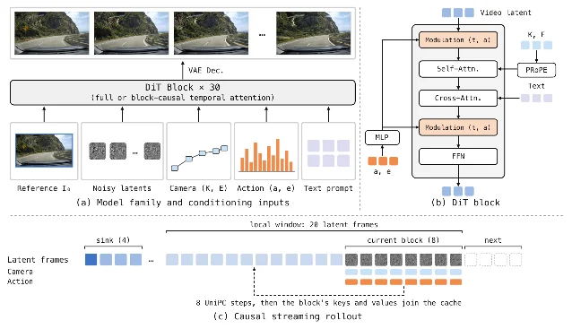
What changes. Video world models are normally shipped as offline generators: you ask for a clip, you wait, you get the whole thing. Astronex-World 1.0 releases a 5B family in two forms — a bidirectional model for full-context generation and a causal model that emits blocks of latent frames one after another and keeps generating — driven by frame-aligned camera trajectories, a continuous action stream and an embodiment identifier, with text events that can be inserted at a chosen point in a rollout. The training claim is unusually modest for the result: all five stages ran on two NVIDIA L20 48 GB GPUs, and the causal model is reported to stream in real time on one. 8
Technical insight. One 30-block video diffusion transformer inherits the Wan2.2-TI2V-5B visual prior and is used with either full temporal attention or block-causal attention. PRoPE injects camera intrinsics and extrinsics into self-attention; the 64-dimensional action vector and its embodiment ID are mapped by an MLP into the same scale, shift and gate modulation that carries the timestep; the text prompt enters through cross-attention. The causal release generates eight latent frames per block with eight UniPC steps, attends to four sink frames plus a 20-latent-frame local window, and appends each finished block's keys and values to a cross-block KV cache — which is what lets a text event change the prompt from a given latent frame onwards without discarding what came before. 8
Quantitative evidence. On WBench, which contains 289 cases and 1,058 interaction rounds across five high-level dimensions, the causal release scores 73.5 on the 158-case navigation subset and 70.0 on the full 289-case set, measured on 832 × 480 video at 24 fps with eight UniPC steps. On the Full set the report places its 5B model above a 13.6B LongCat-Video and a 14B Helios, within one point of a 22B LTX-2.3, and above YUME 1.5, which is post-trained from the same 5B Wan2.2 prior on A100 GPUs. 8
Inspectability. Everything needed to check the claim is out: a project website, a GitHub repository, and released weights. 91011
Caveat. The report lists five limitations of its own. Complex interaction is weak: event editing, subject action and perspective switching go through a text-switch interface that cannot express several independent timed events. Long-horizon drift remains — strong turns, loops and low-light scenes still show colour shift, darkening, structural repainting and detail loss, which the four sink frames and local history only delay. The DMD distillation step appears to suppress motion, in the authors' reading, because stable but near-static solutions are preferred; their own diagnostics place motion amplitude well below the bidirectional model. Physical fidelity is limited: there is no explicit physical state, depth, collision constraint or 3D scene representation, so video coherence is in the authors' own words no proof of accurate physics. Finally, the 64-dimensional action stream and the action-output path are reserved interfaces, meaning driving and robot control spaces connect only through post-training with domain data. 8
Why it matters. Researchers building video world models and embodied agents get an open 5B checkpoint that streams, plus a training recipe that fits on two 48 GB cards. The published limitation list is the useful part: it names colour drift, motion decay and absent physics before you discover them in a rollout.
2. Video DeltaNet: a fixed-size memory for long video context
Team and affiliation. Haocheng Xi, Yiwen Zhang, Kurt Keutzer and Haiwen Feng at the University of California, Berkeley; Yiming Xie, Hexu Zhao, Michael Liu, Thomas Creavin, Xiuyu Li, Zhaoyang Lv and Haiwen Feng at Impossible, Inc.; and Chenfeng Xu at the University of Texas at Austin. arXiv v1 dated 17 September 2026. 4
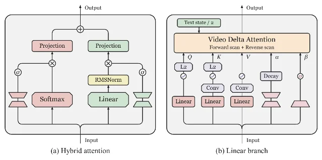
What changes. A video diffusion transformer reprocesses the same long sequence of spatiotemporal tokens at every denoising step, and attention over that sequence is where the time goes. Linear attention would make the cost manageable, but dropping it into a video model directly damages the fine-grained interactions that separate a good clip from a blurry one. Video DeltaNet keeps softmax attention for short-range interactions and for anything involving text or audio, and adds a linear branch with a fixed-size bidirectional memory for long-range video context, so the model's cost stops growing with how much video it has already seen. 12
Technical insight. The linear branch is Video Delta Attention: instead of treating each token separately, it updates memory once per frame, jointly incorporating that frame's spatial tokens, and scans forward and in reverse so information travels in both temporal directions. Separate output projections and learnable gates calibrate how much the two branches contribute, and a staged teacher-alignment recipe introduces the new pathway into a pretrained model a step at a time rather than retraining it. The method is instantiated on MiniMax H3, with the hybrid applied to video-to-video interactions and softmax retained wherever text or audio is involved, combined with eight-step distillation and an SGLang serving stack. 12
Quantitative evidence. Table 2 of the paper measures one 14.3-second 768p clip on B200 GPUs. The 50-step dense H3 model takes 799.6 seconds on a single GPU; 50-step Video DeltaNet takes 307.9 seconds on one GPU, a 2.6× gain from the attention change alone; eight-step distillation brings the same run to 49.3 seconds, 16.2× cumulative; and spreading that across eight GPUs brings it to 6.70 seconds, 119.3× cumulative against the single-GPU dense baseline, which is the number in the abstract. Attention density over the same test falls from 42.08% to 19.98%. On quality, eight-step Video DeltaNet matches or exceeds the 50-step dense model across five no-reference video metrics, and its RAFT motion magnitude is 11.71 pixels against 11.55 for the dense model, while the team's own four-step FastH3 baseline falls to 9.19. 12
Caveat. The 119.3× figure stacks three separate changes — hybrid attention, step distillation, and distributed inference — and only the 50-step comparison isolates the attention gain, which the authors state explicitly by restricting the 50-step variant to the efficiency study. Everything is measured on one backbone and one configuration, a 14.3-second 768p clip. The quality argument rests on no-reference metrics plus endpoint fidelity rather than a reference-based benchmark, and the paper's own fast baseline shows the cost of that trade: FastH3 is the faster student, and it loses motion. The preprint carries no limitations section. 15
Why it matters. Anyone serving a video diffusion model meets this bottleneck, and the change is an architectural one with weights and code attached. The staged teacher-alignment recipe is the transferable part: it is how a linear branch gets added to a model that was already trained without one.
3. MM-Future: generating the futures, then choosing among them
Team and affiliation. Shuai Liu at NIO and the School of Computer Science and Engineering, Sun Yat-sen University; Hechangle Gong at NIO and Beihang University; Hao Jiang, Runlin He, Junxiang Zhan and Sheng Yang at NIO; Shaoqing Ren at NIO and the Artificial General Intelligence Institute, University of Science and Technology of China; and Kai Huang at Sun Yat-sen University. arXiv v1 dated 17 September 2026. 5
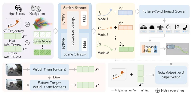
What changes. A driving planner has to commit to one trajectory, but the scene ahead of it has many possible continuations, and world–action models usually connect the two by cascading one into the other or by modelling them jointly in a single direction. MM-Future generates M paired hypotheses, each holding one candidate trajectory and the future scene that would follow it, and lets the scene stream and the action stream interact inside each pair before a scorer ranks the pairs using both the shared history and the imagined future. 16
Technical insight. History is compressed into MM-Tokens by a rank-32 LoRA-adapted DINOv2-S backbone plus a four-layer attention module, at 64 tokens of 256 dimensions per two-frame chunk. A modality-aware diffusion transformer — 16 layers, width 1024 — takes independent scene noise and a structured action prior and co-evolves them through a shared attention block with per-stream AdaLN modulation and separate feed-forward networks. Training uses Best-of-Many supervision with an EMA target encoder; at inference the model samples 64 pairs and runs two Euler steps, scores every pair with a future-conditioned scorer, and returns the highest-scoring trajectory. The operating point is a 2-second history predicting 4 seconds at 2 Hz, from four cameras at 336 × 560. 16
Quantitative evidence. On NAVSIM-v1 navtest, MM-Future trained on the trainval set reaches 94.0 PDMS, which the paper reports as 3.3 points above the strongest world–action baseline, DriveFuture, and 0.3 points above the strongest end-to-end baseline, DrivoR trained on trainval. Under a matched train-only comparison it is 93.4 against 93.1 for DrivoR, which addresses whether the gain is simply extra training data. On NAVSIM-v2 navtest it reaches 91.5 EPDMS, 1.4 points above UniTeD and 1.6 above DriveFuture. In zero-shot closed-loop transfer to HUGSIM over 436 scenarios, without any HUGSIM fine-tuning, it records the highest average HD-Score at 32.3, 3.4 points above Latent-WAM, with its widest margin at Medium difficulty: 51.5 route completion and 40.0 HD-Score, 9.0 and 10.5 points above the strongest baselines. The ablation on hypothesis count is the clearest single result: raising it from one to 32 moves PDMS from 85.1 to 92.9 for paired generation, and from 84.1 to 92.3 for action-only generation. 16
Inspectability. The preprint names no code repository and no project page.
Caveat. The MM-Tokens are implicit, and the authors say so: the scene information they encode is difficult to interpret, and the stated next step is an auxiliary perception module to make the planning-relevant structure visible. Until then the model's planning representation cannot be inspected, which limits failure diagnosis. The margin over the strongest end-to-end baseline is 0.3 PDMS, and evaluation covers NAVSIM-v1, NAVSIM-v2 and HUGSIM. 16
Why it matters. Planning and world-model researchers get a worked design in which hypothesis count and scene–action coupling are separated and ablated, so the two contributions can be judged independently. The result that matters most is the ablation curve, since it shows where the benefit saturates.
4. FlowSGS: splitting the posterior into two steps
Team and affiliation. Tianao Li in the Department of Computer Science at Northwestern University and the NSF-Simons AI Institute for the Sky; Xinhui Qian in the Department of Statistics and Data Science at Northwestern; and Emma Alexander in Computer Science at Northwestern and the institute. arXiv v1 dated 17 September 2026. 6
What changes. Flow matching has become the prior of choice for plug-and-play solvers on inverse problems, but the existing flow-based samplers either assume the forward model is linear or take shortcuts when sampling the posterior. FlowSGS decomposes the posterior with Split Gibbs Sampling into a likelihood step and a prior step, uses Langevin dynamics for the likelihood, and puts a pretrained flow model inside the prior step through the Stochastic Interpolants framework. Because the flow prior's probability paths are straighter than a diffusion model's, the prior step needs fewer network evaluations than a plug-and-play diffusion sampler. 17
Technical insight. The prior step uses Stochastic Interpolants' reverse-time SDE, with a timestep-correction technique that handles the conversion between the likelihood step's noise scale and the flow prior's time variable — the paper's Corollaries 1 and 2 set out the formal relationship to PnP-DM. Sampling alternates the two steps until the chain converges, and the likelihood step is sampled with Langevin dynamics for both linear and nonlinear forward models, which removes the need for a task-specific closed-form inverse. One further experiment swaps in the off-the-shelf Stable Diffusion 3.5 Medium model as a latent-space flow prior. 17
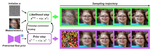
Quantitative evidence. Table 1 averages 100 test images with eight posterior samples per method. On motion deblurring, FlowSGS with a linear interpolant reaches PSNR 29.22, SSIM 0.836 and LPIPS 0.154, against 28.42 / 0.816 / 0.229 for the strongest baseline, FlowDPS, and 28.53 for PnP-DM. On Gaussian deblurring it records 30.09 / 0.847 / 0.141 against FlowDPS at 29.78 / 0.840 / 0.202, and on 4× super-resolution 29.49 / 0.844 / 0.149 against DAPS at 28.99. On compressed-sensing MRI at 8× acceleration it reaches 32.84 PSNR and 0.839 SSIM in the Cartesian sampling pattern and 34.77 / 0.869 in the radial pattern, though its data-fit term of 50.420 is slightly worse than PnP-Flow's 49.892. The nonlinear result is the one to read: on Fourier phase retrieval, where the paper says it is the first flow-based sampler to be benchmarked, FlowSGS reaches 37.52 PSNR, 0.940 SSIM and 0.076 LPIPS with the linear interpolant and 38.45 / 0.950 / 0.056 with the generalised variance-preserving one, against 35.77 / 0.926 / 0.054 for DAPS. That task reports the single best of eight posterior samples rather than the mean. 17
Inspectability. The paper states that model checkpoints trained on CelebA, FFHQ and fastMRI knee are available on its project page, and the preprint text carries no address for that page. No code repository appears in the submission. 17
Caveat. The authors list three limits. Sampling cost is higher than for other flow methods, which they expect one-step flow models to reduce. The experiments cover non-blind inverse problems only, with semi-blind and blind settings left to an EM-style extension. And Langevin dynamics are inefficient with latent-space models, because each step takes a gradient through the decoder — which is why the Stable Diffusion 3.5 experiment is slower than the pixel-space ones, and why the authors propose a hybrid pixel-then-latent scheme. The phase-retrieval numbers use best-of-eight rather than the posterior mean, so they are not directly comparable to the linear-problem columns. 17
Why it matters. Computational-imaging and inverse-problem researchers get a flow-based posterior sampler that does not assume a linear forward model, tested on a genuinely nonlinear task, with the failure mode named. The published limitation about latent-space cost is the practical constraint to weigh first.
5. Paint-Anything: reading a hex value as a colour instruction
Team and affiliation. Ji Xie and Dewei Zhou at ByteDance Seed and Zhejiang University; Xinyu Huang at ByteDance Seed; Zhennan Chen at ByteDance Seed and Nanjing University; and Xun Wang at ByteDance Seed. The submission is a Seed technical report, arXiv v1 dated 17 September 2026. 7
What changes. Asking an image model for a blue logo gives you some blue. A brand needs its own blue. Paint-Anything makes the 24-bit hex value itself the instruction, in one shared prompt interface used for both generating an image and recolouring an object in an existing one, and builds a benchmark to measure whether the delivered colour matches the requested one at the object level. 18
Technical insight. The data pipeline, Paint-500K, starts from real images: a vision-language model grounds the objects a caption refers to, perceptual colour clustering labels them, and editing pairs are synthesised from the result. Shadow makes those labels approximate, so the recipe adds pure-colour anchors whose pixels match their paired hex value exactly — and gates them, activating the anchors only at high-noise timesteps and leaving low-noise training to natural images. That gating is worth 4.75 points on ACBench-T2I and 5.18 on ACBench-Edit over ungated anchors. The accompanying benchmark, ACBench, holds 500 single-object and 500 two-object generation prompts plus 500 real-image recolouring prompts; SAM3 supplies the target mask, the region's mean sRGB is compared with the requested value, and the error is mapped to a 0–100 score where an average channel error of 16 or less scores full marks and 64 or more scores zero. 18
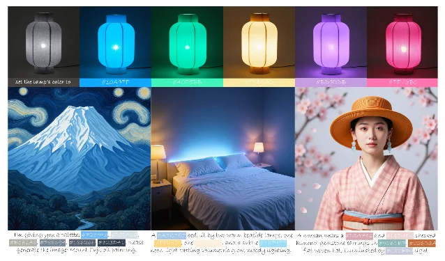
Quantitative evidence. On the FLUX.2-4B base model, fine-tuning with this recipe lifts the ACBench-T2I overall score from 37.02 to 68.58, a relative gain of 85.3%, and ACBench-Edit from 58.90 to 75.57, a relative gain of 28.3%. On the independent CompColor benchmark, which measures compositional colour binding, the scores go from 0.74, 0.70 and 0.73 on the single, close and distant splits to 0.81, 0.80 and 0.76. The same recipe also lifts a 10B model, Z-Image Base, from 33.45 to 53.77 on ACBench-T2I, and the paper reports that the 8B fine-tune outscores the 56B FLUX.2-dev base on both ACBench splits — the 56B model sits at 51.70 for generation and 68.87 for editing. 18
Inspectability. The preprint releases neither code nor weights; the fine-tune starts from a published FLUX.2-4B checkpoint.
Caveat. The authors state that the training data carry no palette-specific supervision and that palette-level control is future work, so multi-colour specifications are handled as several independent object constraints rather than as one palette. The headline percentages are relative to one base model's own score on a benchmark the authors introduce in the same paper, and the metric is a region-mean colour distance, which does not capture a colour gradient across an object. 18
Why it matters. Researchers working on controllable generation and design tooling get a clean demonstration that a numeric colour specification survives being handed to a diffusion model, plus a benchmark and a data recipe to measure colour fidelity against. The reported result that an 8B fine-tune beats a 56B base model on the same task is the most useful single number for anyone deciding where to spend capacity.
What the five have in common
Each of these papers changes one interface between a condition and the generation it drives, and each picks a different place to put it. Astronex-World and Video DeltaNet decide what a video model is allowed to retain: four sink frames plus a 20-frame local window in a cross-block cache, against a fixed-size bidirectional memory updated once per frame. MM-Future decides how many futures the model should hold at once and how to rank them, and its ablation shows the gain running from one hypothesis to 32. FlowSGS and Paint-Anything decide where in the sampling trajectory a constraint binds: alternating likelihood and prior steps until the chain converges, against colour anchors switched on only at high-noise timesteps. The first four all landed on 17 September and all are video or driving models, which reflects what the batch itself contained rather than a turn in the field.
A reading order follows from which interface is your bottleneck:
- Start with Astronex-World 1.0 if you build video world models or embodied agents and want open weights that stream.
- Start with Video DeltaNet if your video diffusion model is slow to serve and you are choosing between attention changes and distillation.
- Start with MM-Future if you work on planning or on world–action models for driving.
- Start with FlowSGS if you work on inverse problems, computational imaging or posterior sampling with a generative prior.
- Start with Paint-Anything if you work on controllable generation, colour specification or design tooling.
References
- 1arXiv cs.CV new listings
arxiv.org
- 2arXiv cs.LG new listings
arxiv.org
- 3Astronex-World 1.0 abstract\
arxiv.org
- 4Video DeltaNet abstract\
arxiv.org
- 5MM-Future abstract\
arxiv.org
- 6FlowSGS abstract\
arxiv.org
- 7Paint-Anything abstract\
arxiv.org
- 8Astronex-World 1.0 technical report
arxiv.org
- 9Astronex-World code
github.com
- 10Astronex-World weights
huggingface.co
- 11Astronex-World project site
world.astronex.com.cn
- 12Video DeltaNet report
arxiv.org
- 13Video DeltaNet code
github.com
- 14Video DeltaNet weights
huggingface.co
- 15Video DeltaNet blog
openvdn.github.io
- 16MM-Future report
arxiv.org
- 17FlowSGS report
arxiv.org
- 18Paint-Anything report
arxiv.org
This story was produced automatically by a channel. One sentence is all it takes for Neodrop to keep producing for you.