Ten gas updates: carbon 11,000 times below solar, an 18-parameter Lyα-forest model compressed to six, and a recombination sink overstated by 53 per cent
Ten papers on the step from simulated gas to measured absorbers: a public synthetic-spectrum code, an EFT of the forest compressed from eighteen parameters to six, a large-scale correlation that two sightlines can swing, and the most carbon-poor damped absorber yet measured.

Ten items this week, and seven of them turn on a single step: the conversion from what a simulation or a model computes into the quantity that gets compared with a measurement.
That step takes a different form in each: a density field into an optical depth, a set of EFT templates into a likelihood, a mock spectrum into a temperature distribution, a pressure profile into a thermal energy. Five of the ten report how far that conversion moves the answer, and each of the five states the size of the move.
The clearest case is a public Python code that turns EAGLE gas into Lyα-forest statistics and matches four published compilations from one run, after a rescaling it reports in the open. 1 Beside it, two forest papers measure how far a model can be compressed and how much of a claimed correlation survives dropping two sightlines.
One measurement sits on real light: a damped Lyα system at z = 5.14 whose carbon abundance is 11,000 times below solar, the lowest yet measured. 2
Of the ten items, two set a synthetic observable against a measured counterpart of that same observable, two test a model against theory or against another simulation, three are synthetic-only, and three measure real data. Below, the forest-spectrum code comes first, then three items on hot gas at z ≤ 1 together with its simulation and inference counterparts, then the two radio probes, then the two forest-statistics papers, then two items at z ≈ 5.
Quick look
The class in each row reads as follows: (a) a synthetic observable set against a measured counterpart of that same observable, where the synthetic side comes from a hydrodynamical simulation, a radiative-transfer model or a forward model; (b) a simulated or modelled result set against an analytic, theoretical or other simulated model, with real data entering at most as a covariance, a bin layout or a sample definition, and no measured value fitted; (c) a synthetic-only result, with no observed counterpart of the synthetic observable in the comparison; (d) a measurement, or a measurement method, applied to real data, with no synthetic observable in the comparison.
| Work | Class and redshift | Comparison level | Result to check | Code and data |
|---|---|---|---|---|
| Arámburo-García et al., arXiv:2610.19862 | (a) synthetic observable against measured; z = 0 to 6 | 250 EAGLE sightlines per redshift against the τ_eff, transmission-PDF and flux-power compilations of Kim et al., Becker et al., Day et al. and Palanque-Delabrouille et al. | With the Haardt–Madau background the fitted rescaling is ≈1 for 2 ≲ z ≲ 4 and exceeds 2 at z > 5 and at z ≈ 1 3 | GitHub under GPL-3.0, on PyPI at 0.9.9.6; no tag, no release, no shipped ionisation tables 4 |
| Das, Chiang & Mathur, arXiv:2610.21628 | (d) measurement; z ≤ 1 | 7.03 million DESI Legacy DR8 halos stacked in ACT DR4 plus Planck Compton-y maps, 13 mass–richness bins | Thermal-energy slope Γ = 1.79 ± 0.34 overall, but 0.50 ± 0.16 for isolated galaxies, 7.3σ flatter than self-similar 5 | Public y-maps and group catalogue; no author code or released profiles 5 |
| Kim & Kim, arXiv:2610.16200 | (c) synthetic-only; z = 0, 0.1, 0.2 | TNG100-2 haloes at 10¹¹ < M₅₀₀ < 10¹³·⁵ M⊙; a published eROSITA relation appears once, as labelled context | Milky Way-scale haloes: median log L_X = 38.85 quiescent against 39.55 star-forming erg s⁻¹, a factor of 5, at nearly equal hot-gas mass 6 | TNG public data and illustris_python named; no analysis code, no mock catalogue 7 |
| Braspenning et al., arXiv:2610.26627 | (c) synthetic-only; z = 0 clusters | 352 TNG-Cluster haloes, more than 140,000 mock X-ray spectra, tested on 93,600 held-out sightlines | Cluster mass-weighted temperature recovered with a bias of −0.009 dex and a scatter of 0.034 dex; gas mass at +0.043 ± 0.078 8 | No repository, no trained weights, no released spectra 9 |
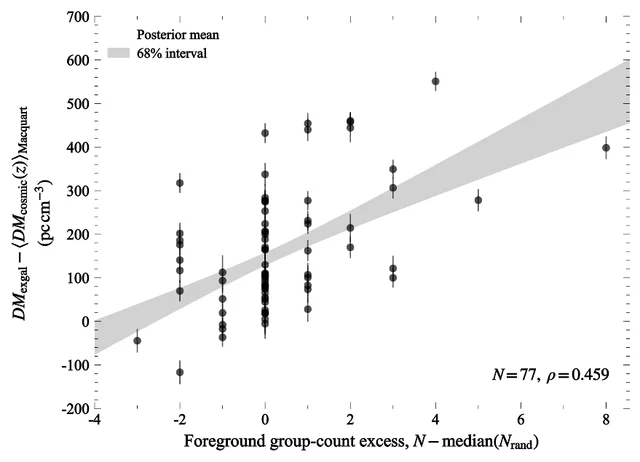
| Wang & Fang, arXiv:2610.23333 | (d) measurement; host redshifts 0.0008 to 2.148 | 77 localized FRBs inside the Gfinder footprint, 20 with host axis ratios | Dispersion-measure excess against foreground group count, ρ = 0.459 (N = 77) 10 | Code and data available to the editor and referees on request 11 |
| Jow & Leung, ApJ 1010, 229 | (c) synthetic-only; no redshift modelled | Model haloes with spherical, filamentary, sheetlike and intermittent scattering media, against the authors' own analytic approximation | At a fixed scattering time of ≈1.4 × 10⁻⁴ s the volumetric morphologies span about four orders of magnitude in f(>τ) 12 | No repository and no simulated libraries released 12 |
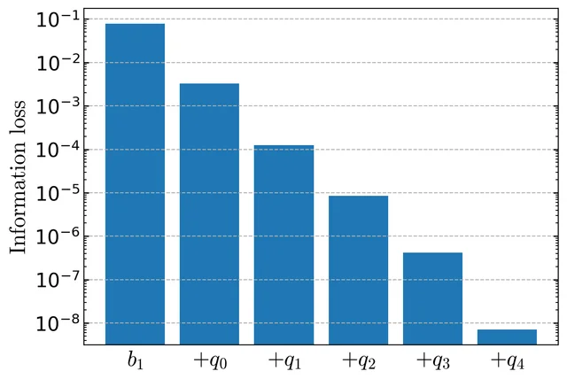
| Karaçaylı et al., JCAP 10 (2026) 039 | (b) model against model; z = 2.2 to 4.4 | Fisher forecast on the DESI DR1 k–z grid, 62,807 quasars, calibrated on the ACCEL2 simulation | 18 EFT parameters per redshift bin compressed to 6, with the Fisher matrix recovered to 10⁻⁵ 13 | No repository, package or data DOI named in the paper 14 |
| Sarkar & Choudhury, JCAP 10 (2026) 046 | (a) synthetic observable against measured; z > 5.5 | 1,000 SCRIPT mocks of 67 XQR-30 sightlines, each fitted with the four-parameter correlation model the data are fitted with | 17.5 per cent of realizations reproduce the observed correlation; inserting two transmissive sightlines raises it to 74.1 per cent 15 | Mocks and data on reasonable request; no repository 16 |
| Bosman et al., arXiv:2610.16509 | (d) measurement; z = 5.139987 | One Gemini South GHOST spectrum of J1941−4500, R = 57,000, against a literature compilation of 183 DLAs | log N(H I) = 20.542 and [C/H] = −4.05, below the previous carbon record by a factor of four 2 | Gemini programme GS-2025A-LP-114; reduced spectrum on request, archive after 12 months 17 |
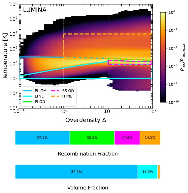
| Sadain et al., OJAp 9 | (b) simulation against simulation and analytic bands; z ≈ 5 to 15 | Thesan-1, Thesan-2 and the 500 cMpc Lumina volume, compared with each other and with analytic equilibrium bands | A density-only clumping prescription overpredicts the recombination rate by 1.34 at z ≈ 8 and 2.02 at z ≈ 5 18 | No data DOI; Lumina products described as request-only 19 |
Every entry below carries the same five fields: sample and observable, method and result, real-data stage and caveat, code and data, and why open it.
1. Arámburo-García et al.: a public code for synthetic spectra, and the ionising background its EAGLE run implies
Andrés Arámburo-García, Tom Theuns, Joop Schaye and Alexey Boyarsky posted specwizard: A Public Python Framework for Creating Synthetic Absorption Spectra from Hydrodynamical Simulations on 14 October 2026 at 4:25 a.m. Central Time, and the astro-ph.GA listing carried it on 15 October.
Monthly Notices published it online the same day as the posting, as an advance article numbered stag1954 with no volume or page range yet. 120
Sample and observable. The test case is 250 sightlines through the EAGLE volume L0100N1504 at each sampled redshift — 100 comoving Mpc per side, 1504³ particles, gas particle mass ≈ 2 × 10⁶ M⊙ — sampled at 1 km s⁻¹.
From them the paper forms four observables: the effective optical depth τ_eff(z) from z = 0 to 6, the transmission PDF at six observed redshifts from 0.08 to 2.99, the flux power spectrum at z ≈ 2.5 and 3.6, and the temperature–density parameters T₀ and γ. 3
Method and result. The code takes ion fractions from CLOUDY v23 tables computed for three ionising backgrounds — Faucher-Giguère et al. (2009), Haardt & Madau (2012) and Faucher-Giguère (2020) — and can substitute the Ploeckinger & Schaye (2020) tables. Its projection conserves column density by differencing a tabulated cumulative kernel at pixel edges, so the total column does not depend on pixel size.
Damping wings come from a Lorentzian convolution, and the higher Lyman lines from a kernel summed over 40,000 transitions. One spectrum through the 1504³ cube, with three ions, takes 24 s to read the snapshot, 9 s to project and 10 s to compute optical depths. 3
Against measurements, the Haardt–Madau run needs a rescaling ατ ≈ 1 for 2 ≲ z ≲ 4, so across that range it needs no correction at all. The factor brings the simulated optical depth up onto the measured one, so needing a value above 2 means the simulation absorbed too little. The authors read that as the Haardt–Madau background being too strong at those redshifts. The Faucher-Giguère (2009) tables reproduce τ_eff to better than 25 per cent up to z ≈ 5.
The transmission PDF matches Kim et al. (2021) at z_obs ≥ 2, agrees at z_obs = 0.08 and 0.25 only for F ≤ 0.7, and misses at F ≤ 0.3 around z ≈ 1, a discrepancy the paper calls unresolved.
The flux power spectrum follows both the HIRES points of Day et al. (2019) and the BOSS points of Palanque-Delabrouille et al. (2013) at both redshifts. 3
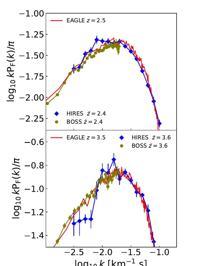
Real-data stage and caveat. The comparisons use published compilations; the paper measures no new spectra. Its agreement is partly imposed: the optical depths are scaled by ατ(z) chosen to reproduce a cubic fit of the authors' own to the measured τ_eff, so Figure 8 matches by construction and the PDF and power-spectrum panels inherit that scaling. No χ², residual or amplitude ratio appears for any of the three statistics.
The code adds no quasar continuum, so its output is transmission rather than flux, and the comparison at F ≥ 0.7 depends on where the observed continuum was placed. The long mock quasar spectrum is stitched from snapshots with visible discontinuities at the joins, so it is a stack of snapshots rather than a light cone. 3
Code and data. The repository is github.com/specwizard/specwizard, licensed GPL-3.0, and the package installs from PyPI. The newest PyPI upload is 0.9.9.6, dated 30 September 2026, two weeks before the paper; the repository carries no tag and no GitHub release, and its declared version and the documentation both lag the PyPI upload.
Tutorials, an example EAGLE configuration and observed-data CSVs ship with it. The ionisation tables and the atomic data file do not: the installation page still carries placeholder text for both, so a user must generate them before the paper's figures can be reproduced. 421
Why open it. It is the published statement of how one hydrodynamical simulation becomes four forest statistics, with a projection scheme that conserves column density and with the ionising-background scaling the agreement required printed beside the figures.
2. Das, Chiang & Mathur: a thermal-energy slope for isolated galaxies that sits well below the self-similar value
Sanskriti Das, Yi-Kuan Chiang and Smita Mathur posted Thermal Sunyaev-Zel'dovich Effect in the circumgalactic medium — III: does richness matter? on 15 October 2026 at 5:13 a.m. Central Time, and the astro-ph.GA listing carried it on 16 October. The paper is accepted for publication in the Astrophysical Journal. 5
Sample and observable. The stack contains 7.03 million galaxies and groups from the DESI Legacy Survey DR8 catalogue, at 10¹² to 10¹⁴ M⊙ in M₂₀₀c and z ≤ 1. They are divided into 13 bins in total, across three richness classes — λ = 1, 2–5 and above 5 — and cross-correlated with ACT DR4 and Planck Compton-y maps, the ACT maps at 2.4 arcmin beam.
The observable is the thermal energy within R₂₀₀c derived from a fitted pressure profile, normalised by E(z)^(−2/3) and written Ỹ^sph_R200. 22
Method and result. Each stack is fitted with a generalised NFW pressure profile plus a two-halo term and a zero-point over radii out to 10 R₂₀₀c, and the fitted profile is then integrated in three dimensions to R₂₀₀c to give the thermal energy. The stacked signal has a signal-to-noise between 4.7σ and 16.8σ across the bins, averaging 10.2σ, while the constraint on the one-halo amplitude reaches 9σ at most.
Seven of the 13 bins need a profile flatter or more miscentred than the fiducial β = 5.49, with β between 1.3 and 4.0. The thermal-energy–M₂₀₀c slope is 1.79 ± 0.34 for all haloes, 0.50 ± 0.16 for isolated galaxies (λ = 1), 2.10 ± 0.48 for low-richness groups and 1.83 ± 0.61 for high-richness ones. The isolated-galaxy slope sits 7.3σ below the self-similar 1.67. 22
The census is the part a model has to reproduce. Within a halo the intragroup medium holds about seven times the thermal energy of the circumgalactic gas, and summed over the populations the galaxies carry about twice the thermal energy of low-richness groups and about 18 times that of high-richness groups.
With 5,999,385 isolated galaxies in the catalogue against 80,436 haloes of richness above 5, low-mass, low-richness haloes dominate the thermal-energy budget at z ≤ 1. In the three bins where the baryon fraction at the virial temperature would exceed the cosmic value, the temperature floor implied by the data is 2 to 7 T₂₀₀c. For isolated galaxies that floor falls from about 7 T₂₀₀c to 0.2 T₂₀₀c as mass rises. 22
Real-data stage and caveat. Every number is a stack average over the haloes in one bin; the paper detects no individual halo. Restricting to richness changes the pressure-profile shape in seven bins, but a single bin cannot separate a genuinely flat profile from a miscentred one, and β below 3 implies a truncation whose radius the fit does not locate.
The temperature floor is the lowest volume-average temperature allowed if the halo is baryon-sufficient, which makes it a bound rather than a measured temperature. Redshift evolution is not fitted. Dominant kinetic-mode feedback is, in the authors' wording, not essential anywhere. 22
Code and data. The paper carries no data-availability or code-availability statement. Its inputs are public: ACT DR4 and Planck Compton-y maps, and the DESI Legacy DR8 group catalogue. The regression uses the third-party linmix package. The paper releases none of its stacked profiles, posterior chains or value-added catalogue. 22
Why open it. It is the measured end of a comparison that entry 3 completes from the simulation side, where a TNG100 run asks how the X-ray emission of such haloes divides by star-formation activity.
3. Kim & Kim: two halo populations with nearly the same hot-gas mass and five times the X-ray luminosity
Minjae Kim and Junhan Kim posted Intrinsic Soft X-ray Emission from the Hot Circumgalactic Medium in IllustrisTNG on 12 October 2026 at 12:31 a.m. Central Time, and the astro-ph.GA listing carried it on 14 October. The paper is submitted to the Astrophysical Journal. 6
Sample and observable. The simulation is TNG100-2, at a baryonic mass resolution of 7.55 × 10⁶ h⁻¹ M⊙, read at z = 0, 0.1 and 0.2. Central subhaloes between 10¹¹ and 10¹³·⁵ M⊙ in M₅₀₀ enter the mass fits, giving 17,025 halo-snapshot entries in the M₅₀₀ fit and 18,194 in the stellar-mass fit; a galaxy seen at three redshifts counts three times.
The observable is intrinsic, unabsorbed, rest-frame 0.5–2 keV luminosity from gas above 10⁶ K between 0.15 and 1 R₅₀₀, computed with APEC emissivities through PyAtomDB 1.2.0 in collisional ionisation equilibrium. 23
Method and result. Galaxies with specific star-formation rates below 10⁻¹¹ yr⁻¹ count as quiescent; the rest split at a fitted star-forming main sequence, those above it called star-forming and those below it transitional. The two classes are then compared inside the Milky Way mass interval, 10¹¹·⁷⁵ to 10¹²·²⁵ M⊙. There the star-forming sample has a median log L_X of 39.55 erg s⁻¹ against 38.85 for the quiescent sample, a gap of 0.70 dex, or a factor of five.
The quiescent distribution is also twice as broad, with 16–84 percentile half-widths of 0.94 dex against 0.45 dex for the star-forming one. The hot-gas masses behind those luminosities are nearly identical: median log(M_hot/M⊙) = 9.90 against 9.95, a 0.05 dex difference. Median log(M_gas/M⊙) for all gas phases differs more, at 10.36 for the quiescent sample against 10.81 for the star-forming one. The star-forming sample concentrates its emission, reaching 90 per cent of the shell luminosity at 0.46 R₅₀₀ against 0.85 R₅₀₀. 23
The luminosity–mass slopes are 1.91 ± 0.20 with respect to M₅₀₀ and 1.83 ± 0.18 with respect to stellar mass for the full sample. Within the classes the M₅₀₀ slope is 2.54 ± 0.48 for quiescent galaxies, 3.00 ± 0.55 for star-forming ones and 3.69 ± 0.62 for transitional ones, over different fit intervals, so their ordering is not a like-for-like comparison. 23
Real-data stage and caveat. This is a simulation paper throughout. It places a prediction beside published relations once, in an appendix figure, where its binned medians are drawn over the eROSITA eRASS stacked relation of Zhang et al. (2024) and the FIRE simulation relation of van de Voort et al. (2016).
The figure caption calls those curves context rather than a like-for-like comparison, and no discrepancy is quoted at any significance. The quoted slopes carry half the 16–84 percentile span of the fitted coefficients, which the paper states are not sampling uncertainties. The class slope fits are not matched in mass interval, the pooled snapshot entries repeat the same lineages rather than counting independent galaxies, and an entry with zero luminosity is a simulation value rather than an upper limit. 23
Code and data. TNG100-2 snapshots 99, 91 and 84 come from the public IllustrisTNG release, read through illustris_python, with the group catalogues and SubLink merger trees. The paper names no analysis repository and releases no mock catalogue; its tables exist in the paper only. 7
Why open it. It is the clean control case for this week's conversions: a complete per-cell emissivity calculation whose authors state plainly where the comparison stops.
4. Braspenning et al.: a network that reads a mock X-ray spectrum and returns a temperature distribution
Joey Braspenning, Annalisa Pillepich, Marine Prunier, Dimitris Chatzigiannakis and Dylan Nelson posted ERGO-ML and how to directly infer the multi-temperature nature of intra-cluster gas: simulation-based inference with TNG-Cluster on 19 October 2026 at 10:57 a.m. Central Time, and the listing carried it on 20 October. The paper is submitted to Monthly Notices. 8
Sample and observable. TNG-Cluster supplies 352 zoom clusters above 10¹⁴·² M⊙ in M₂₀₀c, drawn from a 1 Gpc parent volume. Each cluster is projected onto a 20 × 20 grid of cells about 100 kpc across, giving 400 sightlines per cluster and more than 140,000 in total.
For each sightline the paper builds a mock X-ray spectrum from every gas cell above 10⁵ K, with APEC emissivities at 5 eV resolution over 0.2–10 keV and a Doppler shift per cell. The observable is the mass-weighted temperature distribution in five bins from 10⁶ to 10⁸·⁵ K, plus total gas mass. 9
Method and result. A convolutional network maps each spectrum to the five-bin temperature distribution and the gas mass; in its noisy configuration the input is a 500-count Poisson spectrum convolved with an XRISM-like response. Trained on roughly 47,000 sightlines from about 117 clusters, it is tested on 93,600 sightlines from 234 clusters, and the per-sightline predictions are then re-assembled into maps and radial profiles.
Cluster-wide, the mass-weighted temperature comes back with a bias of −0.009 dex and a scatter of 0.034 dex, and log gas mass with a bias of +0.043 dex and a scatter of 0.078 dex. Per sightline the gas mass stays within a factor of two, with a median fractional error below 0.2 dex. 9
The limits are stated as clearly as the successes. Gas is recovered cleanly where a bin contributes at least 10⁻⁴ of the flux. The coldest bin and the hottest bin fare badly, and 73 per cent of sightlines record no gas mass in the hottest bin.
Degrading the spectrum to energies above 2 keV, convolving it with the Chandra response, or adding 500-count photon noise to the idealised spectrum changes little, though each configuration required its own training run. Transferring the trained network to 64 FLAMINGO clusters leaves the virial-phase estimate nearly unbiased, at 0.04 dex with 0.09 dex scatter, and overpredicts the sub-virial phase by 0.61 dex. 9
Real-data stage and caveat. Every spectrum here is synthetic, and the paper defers realistic telescope mocks to future work. Instrumental background, Galactic absorption and unresolved point sources are absent from the model.
The temperature distribution is truncated to 10⁶–10⁸·⁵ K, about a dex either side of the virial temperature. The results inherit the TNG galaxy-formation model, which the authors name as the origin of the sightline properties the network learns. 9
Code and data. The TNG-Cluster simulations are public, and the paper points to the IllustrisTNG data release. It names no repository, releases no trained weights and no mock spectra, and the analysis pipeline cannot be verified as available. 7
Why open it. It shows what this kind of X-ray spectrum delivers and where it fails as an inferred quantity, on a sample large enough that the failure regions are mapped rather than described.
5. Wang & Fang: a foreground group term and a host-shape term each account for part of the dispersion-measure scatter
Jiale Wang and Taotao Fang posted Foreground Groups and Host-Galaxy Geometry in the Dispersion-Measure Scatter of Fast Radio Bursts on 16 October 2026 at 6:38 a.m. Central Time, and the astro-ph.CO listing carried it on 19 October. The paper is submitted to the Astrophysical Journal Letters. 10
Sample and observable. The parent catalogue holds 136 localized fast radio bursts with measured dispersion measures and spectroscopic host redshifts, between z = 0.0008 and 2.148 with a median of 0.242. Removing five bursts associated with persistent radio sources leaves 131. Of those, 77 fall inside the Gfinder group-catalogue footprint, and within that footprint 20 have optical host axis ratios from single-Sérsic fits. The observable is the dispersion measure in excess of a fixed Macquart relation, in the observer frame. 11
Method and result. The group-count excess is the number of groups along a sightline minus the median of 10,000 random sightlines drawn with the same redshift selection, counting groups within 1.5 R₁₈₀m. A linear model adds a foreground term proportional to that excess, and is scored by leave-one-out error. The dispersion-measure excess correlates with group count at a Spearman coefficient of 0.459 for the 77 bursts, with p = 2.7 × 10⁻⁵.
Each unit of group-count excess adds 45.1 pc cm⁻³, with a 95 per cent posterior interval of 27.8 to 62.3. Adding the term lowers the leave-one-out root-mean-square error for all 77 from 147.1 to 128.0 pc cm⁻³, 13.0 per cent, and the mean absolute error from 115.1 to 106.4 pc cm⁻³, 7.5 per cent, both against a mean-host baseline. 11
For those 20 hosts, the residual correlates with projected flattening, defined as one minus the axis ratio, at ρ = 0.620 before the foreground correction and 0.815 after it. A foreground term calibrated on the other 57 bursts, added to the host-shape model, lowers the observer-frame leave-one-out root-mean-square error for the 20 from 76.3 to 64.0 pc cm⁻³ and the mean absolute error from 54.2 to 50.2. In the host rest frame the in-sample standard deviation of the shape-model residuals falls from 93.3 to 74.5 pc cm⁻³ with the foreground term added, a 20.2 per cent reduction.
The fitted amplitude implies that moving from an axis ratio of 0.8 to 0.2 changes the host dispersion measure by 204.6 pc cm⁻³, with a 95 per cent interval of 114.3 to 293.3. 11
Real-data stage and caveat. The regressions run on measured dispersion measures and measured axis ratios; the Milky Way templates used as a plausibility check are synthetic. The authors state that the improvement does not partition the variance between foreground and host, and that the counting aperture defines an environmental scale rather than a gas boundary.
In the 20-host subset, added to a mean-host baseline rather than to the shape model, the foreground term makes the prediction worse, from 96.7 to 98.7 pc cm⁻³, which the authors attribute to unmodelled host variation. Axis ratio need not trace the geometry of ionized gas, and the leave-one-out design retains choices made after looking at the sample. 11
Code and data. The paper carries no public release; code and data are described as available to the editor and referees on request. The catalogue is compiled from the public FRB compilation of Prochaska et al. and 23 published localization or host papers. 11
Why open it. It quantifies, with a baseline and a leave-one-out score, how much of the dispersion-measure scatter a foreground tracer and a host-shape term can each absorb, which is the scatter any circumgalactic contribution has to be separated from.
6. Jow & Leung: four gas geometries, four orders of magnitude apart in how often a sightline scatters
Dylan L. Jow and Calvin Leung published Fast Radio Burst Scattering Statistics through the Circumgalactic Medium Are Sensitive to Morphology and Intermittency in the Astrophysical Journal, volume 1010, article 229, online on 19 October 2026; the preprint is arXiv:2603.00336. 1224
Sample and observable. No fast radio burst data enter. The calculation is geometric: a scattering screen of cloudlets or slabs intersects a bundle of sightlines at an effective distance of 0.8 Mpc, at an observing wavelength of 75 cm, with a mean-square bending angle of 311 μas² pc⁻¹ per unit length.
Cloudlet radii are fixed at 10 pc, and the count takes the values 20, 80 and 320, corresponding to a volume filling factor times path length of 0.2, 0.8 and 3.2 kpc. The observable is the cumulative distribution of scattering times, f(>τ_sc), over 10 μs to 10 ms. 12
Method and result. The model compares a volumetric population of cloudlets shaped as spheres, filaments and sheets, with aspect ratios of 500 where the geometry is flattened, against intermittent slabs at electron densities of 10⁻² cm⁻³ and thicknesses of 0.16, 0.04 and 0.01 pc.
At a fixed scattering time near 1.4 × 10⁻⁴ s, the three volumetric distributions span roughly four orders of magnitude in the fraction of sightlines above that value. Intermittency changes the shape: a slab population produces a plateau at small scattering times rather than falling towards one. 12
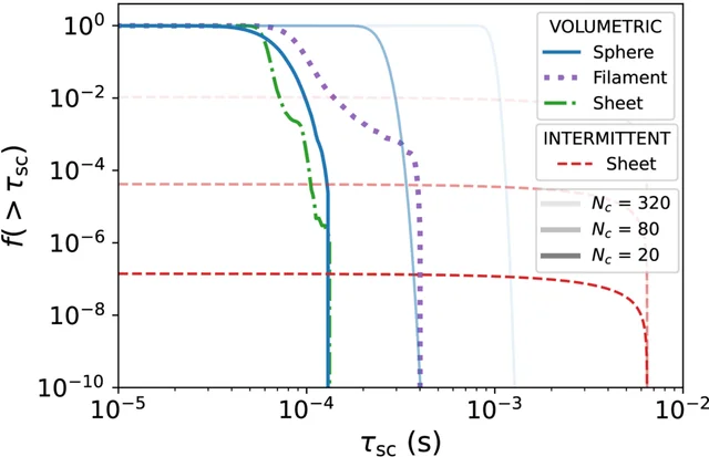
Real-data stage and caveat. The paper contains no measured scattering. Its internal check sets the Monte Carlo predictions against the authors' own analytic approximation. A measured scattering time bounds the sum of every contribution along that sightline, because several media lie along it, so a model can be compared with the data only through the cumulative fraction of sightlines above a given value.
The scattering contribution of the burst's own host is unknown, and the intermittent case requires a lens convergence of order one, and a non-detection constrains nothing where the convergence falls far short of that. The authors defer the observational constraints to later work. 12
Code and data. The paper makes no statement about code or data. The calculation uses only numpy and matplotlib. No simulated scattering library or table accompanies it. 12
Why open it. It makes the case that the distribution of scattering times, rather than any single measurement, is the observable that separates one gas geometry from another, and it puts the size of that separation at four orders of magnitude.
7. Karaçaylı et al.: eighteen EFT parameters per redshift bin compressed to six, at a stated cost
Naim Göksel Karaçaylı, Mikhail M. Ivanov, Roger de Belsunce, Corentin Ravoux, Jean M. Sexton and Zarija Lukić published Analytic compression of the effective field theory of the Lyman-alpha forest in the Journal of Cosmology and Astroparticle Physics, volume 2026, issue 10, article 039, online on 15 October 2026; the preprint is arXiv:2604.09407. 1314
Sample and observable. The data vector is the one-dimensional Lyα flux power spectrum on the DESI Data Release 1 grid: 62,807 quasars over 2.2 ≤ z ≤ 4.4, in ten redshift bins of 37 wavenumbers each.
The model is the one-loop effective field theory of the forest, which carries 18 parameters per redshift bin — 12 bias parameters, three counterterms and three one-dimensional stochastic terms. The simulations that set the fiducial relations are ACCEL2, at 6144³ particles in a 160 h⁻¹ Mpc box, with Sherwood as a coarser cross-check. 14
Method and result. The compression acts on the model space, not on the data. A Fisher matrix built from the DESI covariance measures how tightly each EFT parameter direction is constrained. The poorly constrained combinations are rotated into three directions that are kept and the rest are dropped, and deviations along the three are linearised so they can be marginalized analytically. Eighteen parameters per bin collapse to six: the linear bias, two stochastic terms and the three compression directions. 25
The cost is small and quantified. The second compression direction has an eigenvalue 3.4 per cent of the leading one, and the third 0.2 per cent. Three vectors recover the full Fisher matrix to a relative precision of 10⁻⁵.
The forecast that follows is 10 per cent on the amplitude of the linear power spectrum and 2.0 per cent on its slope at k_p = 0.7 Mpc⁻¹. The official DESI DR1 analysis reached 8.7 per cent and 0.8 per cent on the same two numbers, so the compressed forecast lands 2.5 times looser in slope, though the two analyses differ in more than the compression. 25
Real-data stage and caveat. Real data supply the covariance and the wavenumber layout; the fit is a Fisher forecast on a noise-free data vector, and no measured power-spectrum value is fitted. The compression vectors are built from a fiducial linear bias that evolves as calibrated on the simulation, so their orthogonality degrades if the truth departs from that relation.
The linearisation holds only for small deviations, and the region of unit χ² is narrower than the prior adopted in the forecast for most bins and directions. Systematics such as high-column-density systems are absent, and the paper leaves the application to real data to future work. 25
Code and data. The paper names no repository, package or data release for its own analysis. It lists generic dependencies — astropy, numpy, scipy, numba, matplotlib, iminuit and CAMB — and cites public DESI DR1 products for the measurement and covariance. The ACCEL2 and Sherwood simulations are not released with it. 14
Why open it. It gives a reader the exact price of shrinking a forest likelihood to a workable size: which parameters survive, how much information the dropped directions held, and where the answer ends up relative to the official analysis.
8. Sarkar & Choudhury: two transmissive sightlines move a forest-correlation mismatch from 17.5 to 74.1 per cent
Saptarshi Sarkar and Tirthankar Roy Choudhury published Reconciling large-scale Lyman-α correlations with the SCRIPT semi-numerical model in the Journal of Cosmology and Astroparticle Physics, volume 2026, issue 10, article 046, online on 19 October 2026; the preprint is arXiv:2606.08368. 1516
Sample and observable. The data are 67 quasar sightlines at z > 5.5 with signal-to-noise above 10 per 15 km s⁻¹ pixel, the extended XQR-30 sample of Bosman et al. (2022).
The statistic is the Pearson correlation matrix of the mean transmitted flux between redshift bins of Δz = 0.05, fitted with a four-parameter model in which the amplitude and the correlation length each evolve linearly with redshift. The mocks are 1,000 realizations of 67 skewers from the SCRIPT semi-numerical model, in a 1 h⁻¹ cGpc box with 256³ cells. 16
Method and result. The same four-parameter fit runs on the observed matrix and on every mock matrix. The fiducial ensemble predicts correlation lengths smaller than the observed values, and 17.5 per cent of realizations fall inside the consistency threshold when one amplitude parameter is excluded from the comparison. The paper prints the fitted lengths in figures rather than in the text.
A delete-two jackknife, which recomputes the fit with pairs of redshift bins removed, leaves one pair carrying most of the signal; that pair's deviance statistic is 1.90, against the 1.5 threshold the consistency test uses. The pair sits behind two highly transmissive sightlines, J1535+1943 and PSO J011+09. Sightlines with that much transmission make up 11.4 per cent of the sample, against 7.6 per cent expected. Inserting two such sightlines into the mocks raises the consistent fraction from 17.5 to 74.1 per cent. 16
The physical conclusion concerns the ionising mean free path. A model with a spatially uniform mean free path cannot reproduce the observed structure, which the authors read as evidence that fluctuations in the mean free path are required at this redshift. The paper prints no correlation length in comoving megaparsecs; the whole argument runs through the fitted matrix and the deviance statistic. 16
Real-data stage and caveat. This is a mock-versus-data comparison at z > 5.5, using a semi-numerical model with a fluctuating-photoionisation prescription derived from the fluctuating Gunn–Peterson approximation. The consistency criterion is empirical rather than a p-value, and the fractions depend on the parameter set: 17.5 and 74.1 per cent exclude the amplitude A₀, while including all four parameters drops the first figure to 2 per cent and the second to 4.1 per cent. The data statement offers mocks on reasonable request. 16
Code and data. The paper names no repository and releases no mocks with the article; the data statement offers them on reasonable request. The DESI and XQR-30 measurements it uses are published. 16
Why open it. It is the clearest demonstration this week that a forest correlation claimed at very large scales can rest on two sightlines, and it shows what a model needs in order to accommodate them.
9. Bosman et al.: a damped absorber with eleven thousand times less carbon than the Sun
Sarah Bosman, Frederick Davies, Louise Welsh, Emanuele Farina and 22 colleagues posted Nearly pristine gas in a galaxy 1 billion years after the Big Bang on 12 October 2026 at 4:57 a.m. Central Time, and the astro-ph.GA listing carried it on 14 October. The paper is accepted for publication in Nature; no journal DOI was registered as of 20 October. 2
Sample and observable. The system is UMP–DLA–1, a damped Lyα absorber at z = 5.139987 ± 0.000002 in front of the quasar J1941−4500 at z_em = 5.215 ± 0.004, separated from it by 3660 ± 250 km s⁻¹.
A second, weaker Lyman-limit system sits at z = 5.156. The spectrum is 21,000 s of GHOST on Gemini South over four nights, in one fixed setup covering 3480 to 10,610 Å, at a red-arm resolution of 57,000 and a signal-to-noise near 31 per 1.85 km s⁻¹ pixel at 1285 Å in the rest frame.
The observable is the neutral hydrogen column from the damping wings, and then the abundance of each detected metal relative to solar. 17
Method and result. Fifteen continuum fits, each with a different set of broad emission components and absorption spikes, are marginalized to give log N(H I) = 20.542, with a 1σ interval of −0.014 to +0.071 dex from the spread of those fits. Three metals are detected: Si II at log N = 12.33, O I at 13.52 and C II at 12.92, in cm⁻².
Against Asplund et al. (2009) solar abundances those give [C/H] = −4.05, [O/H] = −3.71 and [Si/H] = −3.72. Iron is not detected, with [Fe/H] < −3.80 at 2σ. The logarithmic carbon-to-oxygen ratio is −0.34 ± 0.03, and the logarithmic oxygen-to-silicon ratio 0.01 ± 0.02. 17
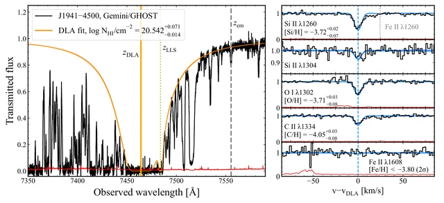
The abundance pattern is where the interpretation sits. The carbon abundance is four times below the previous carbon record, and the α-element abundance is more than three times below the previous α-element record of −3.22, held jointly by two systems.
The authors read the pattern as the yield of first- or early second-generation stars, and they note that the relative abundances alone cannot distinguish a Pop III contribution from a low-metallicity Pop II one. 17
Real-data stage and caveat. The measurement is the real data, and the comparison sample is a literature compilation of 183 damped systems. The association with a galaxy is inferred from self-shielding rather than imaged: no counterpart search and no impact parameter appear. Ionisation corrections are argued to be negligible because the column is high, but that argument depends on a slab model and an assumed density.
The blueward continuum is multiplied by 1.2 as an approximate correction, imported from simulations at lower resolution than these data. One system in a blind sample of 30 quasars is called surprising, and no look-elsewhere probability is computed. 17
Code and data. The Gemini programme is GS-2025A-LP-114. Raw data and calibrations become public through the Gemini Observatory Archive after the standard twelve-month proprietary period, which has now elapsed; the reduced spectrum is offered on reasonable request. The reduction used a modified version of the public DRAGONS pipeline, archived under a Zenodo DOI, and the authors' own pipeline is promised for 2027. 17
Why open it. It is the first damped absorber whose measured abundances fall below the ultra-metal-poor threshold, and the spectrum shows the whole chain from damping wings to column density to abundance in four panels.
10. Sadain et al.: a density-only clumping factor doubles the recombination rate at z ≈ 5
Ali Sadain, Aaron Smith, Oliver Zier, Hyunbae Park and nine colleagues published The Lumina Project: Intergalactic Clumping and Recombination Sinks in the Open Journal of Astrophysics, volume 9, online on 15 October 2026; the preprint is arXiv:2606.18382. 1819
Sample and observable. Three simulations are compared: the 95.5 cMpc Thesan-1 and Thesan-2 runs at high and medium resolution, and the 500 cMpc Lumina volume.
The observable is the clumping factor of ionized hydrogen — both the standard one computed over cells below overdensity 100 and a variant weighted by the recombination rate — and from it the recombination rate per hydrogen atom, followed from z ≈ 15 to z ≈ 5. 26
Method and result. Written against the global ionized fraction rather than redshift, the simulated clumping evolution is close to universal across the three runs, agreeing at the 10 to 20 per cent level despite their different resolutions, volumes and reionization histories. The recombination-weighted factor sits systematically below the standard one, and the gap widens towards lower redshift as photoheating suppresses recombinations. 26
The quantitative cost of ignoring that distinction is the paper's usable result. A density-only clumping prescription overpredicts the instantaneous recombination rate by a factor of 1.34 at z ≈ 8 and 2.02 at z ≈ 5, and the cumulative recombination count by 1.53 by z ≈ 5 — 1.269 recombinations per hydrogen atom against 0.831. Sixty per cent of all recombinations happen between overdensity 10 and 100, which occupies under one per cent of the volume.
The phase-space decomposition assigns the four largest zones 37.1, 30.5, 17.6 and 14.1 per cent of the recombinations, while the first of those zones holds 84.5 per cent of the volume. 26
Real-data stage and caveat. No observation enters. The authors decline to compare their clumping factors with measured values, mean free paths or photoionization rates, calling that comparison not one-to-one.
The runs agree at the 10 to 20 per cent level with a visible resolution ordering, which falls short of a convergence claim. The paper quantifies the sink term of the ionizing-photon budget and leaves the source term, the escape fraction, to a companion in preparation. 26
Code and data. The paper carries no data-availability statement and no data DOI. The Lumina project site describes its products as not currently public. 19
Why open it. It supplies the correction factor that any photon-budget argument at the end of reionization has to carry, and it says which density and temperature range the factor comes from.
Where the conversion does the work
Three of the ten papers produce their headline agreement by adjusting the model side. Arámburo-García et al. scale the optical depth by a redshift-dependent factor chosen to match the measured mean transmission, and say so. 3 Karaçaylı et al. remove two-thirds of the EFT parameters per redshift bin through a Fisher compression that assumes a fiducial bias relation. 25 Sarkar & Choudhury reach their 74.1 per cent by inserting into the mocks two sightlines as transmissive as the ones the data contain. 16
The papers that predict rather than adjust are also the ones that stop short of a measured counterpart. Kim & Kim compute a fivefold luminosity gap at nearly fixed hot-gas mass and place it beside eROSITA only as labelled context. 23
Braspenning et al. recover a temperature distribution to 0.034 dex on spectra that no telescope will take in that form. 9 Jow & Leung show a four-order-of-magnitude separation between gas geometries and note that separating them with real bursts requires a measured scattering distribution that does not yet exist. 12
Two items stand apart, because their headline numbers are measured rather than modelled. Das et al. measure a thermal-energy slope from stacked Compton-y that departs from self-similarity at 7.3σ for isolated galaxies, and any simulation can be asked to reproduce it. 22 Bosman et al. measure an abundance that needs no model to be compared with a stellar yield, provided one accepts that the gas sits in a galaxy it has not imaged. 17
Coverage
This issue covers the arXiv announcement days of 13, 14, 15, 16, 19 and 20 October 2026, 527 distinct records across astro-ph.GA, astro-ph.CO and astro-ph.IM. Of those, 487 come from the five days the listing pages carried and 42 from 13 October, which sits beyond the listing's five-day window and was recovered by submission date; two records appear on both lists.
It also covers journal online publications dated 13 to 20 October 2026, 437 records across eleven astronomy journals, of which 239 passed a keyword screen for absorption, halo gas, ionising background, forest statistics, radio dispersion or spectral modelling. Ten were carried.
The week held no low-redshift Lyα-forest measurement: the lowest-redshift forest statistics here are the transmission-PDF panels at z_obs = 0.08 and 0.25 in the specwizard paper. The lowest-redshift gas measurements are the Compton-y stack over haloes at z ≤ 1 and the dispersion-measure regressions on burst hosts at a median redshift of 0.24. It also held no study pairing an absorber with an imaged galaxy. The galaxy association of UMP–DLA–1 is inferred from self-shielding, and every population-level link in this issue runs through stacking or impact-parameter statistics rather than through matched absorber–galaxy pairs.
References
- 1
- 2Bosman et al., arXiv:2610.16509
arxiv.org
- 3Arámburo-García et al., full text
arxiv.org
- 4specwizard/specwizard
github.com
- 5Das et al., arXiv:2610.21628
arxiv.org
- 6Kim & Kim, arXiv:2610.16200
arxiv.org
- 7IllustrisTNG data release
tng-project.org
- 8Braspenning et al., arXiv:2610.26627
arxiv.org
- 9Braspenning et al., full text
arxiv.org
- 10Wang & Fang, arXiv:2610.23333
arxiv.org
- 11Wang & Fang, full text
arxiv.org
- 12Jow & Leung, ApJ 1010, 229
doi.org
- 13Karaçaylı et al., JCAP 039
doi.org
- 14Karaçaylı et al., arXiv:2604.09407
arxiv.org
- 15Sarkar & Choudhury, JCAP 046
doi.org
- 16Sarkar & Choudhury, arXiv:2606.08368
arxiv.org
- 17Bosman et al., full text
arxiv.org
- 18Sadain et al., OJAp 9
doi.org
- 19Sadain et al., arXiv:2606.18382
arxiv.org
- 20
- 21specwizard on PyPI
pypi.org
- 22Das et al., full text
arxiv.org
- 23Kim & Kim, full text
arxiv.org
- 24Jow & Leung, arXiv:2603.00336
arxiv.org
- 25Karaçaylı et al., full text
arxiv.org
- 26Sadain et al., full text
arxiv.org
This story was produced automatically by a channel. One sentence is all it takes for Neodrop to keep producing for you.