Five diffusion papers from the September 25 batch: routing between two model sizes, a self-calibrating Bayesian score, and decoupled audio–video rewards
A ranked scan of five diffusion-model preprints from the September 25, 2026 arXiv batch: training-free routing between a large and a small model along a video-denoising trajectory, generator-only few-step video post-training, a condition-aware training regularizer, a guidance rule that calibrates itself, and reinforcement learning that gives each modality tower its own turn.

arXiv's newest announcement is the batch for Friday, 25 September 2026: 111 new
cs.CV submissions and 119 new cs.LG submissions, covering the submission cycle that closed with arXiv's 24 September 2026 cutoff. 12 A listing page groups everything announced together, and a section header says nothing about when an individual entry was written, so every candidate was checked against the arXiv API one identifier at a time. All five papers below carry verified v1 timestamps of 23 or 24 September 2026 (UTC), the latest at 17:48 on 24 September.Citation momentum still cannot rank anything at this age. An OpenAlex lookup by arXiv DOI answered for all five identifiers this run — HTTP 200, where earlier runs met HTTP 404 — and returned a citation count of zero with no yearly history for each of them. 3 Semantic Scholar's graph API returned HTTP 429 on every identifier. 4 The ordering below therefore rests on method novelty, author-reported evidence, disclosed affiliation and public inspectability. Every number in this digest is author-reported unless a sentence says otherwise.
The five at a glance
| Rank | Paper | Central move | Strongest reported signal | Inspectability |
|---|---|---|---|---|
| 1 | TRACK | Routing each denoising step to a large or a small model, from a disagreement map computed offline | 1.95×–2.73× faster sampling across four released video pipelines, with VBench temporal metrics level with or slightly above the all-large baseline 5 | No code in the preprint |
| 2 | ViRDM | Dropping the teacher and the critic, and post-training only the generator against a fixed representation distribution | VBench total 84.87 against 84.51 for the strongest four-step causal baseline, with peak memory down from 77.1 GB to 48.3 GB per GPU 6 | Project page only |
| 3 | CARE | Scaling the representation penalty by how similar two samples' conditioning signals are | SiT-XL/2 reaches at 2.4M steps an FID below the baseline at 7M steps; FID 17.19 → 13.91 at 400k steps 7 | No code in the preprint |
| 4 | FB-GDM | Inferring the two guidance precisions of an inverse-problem sampler instead of tuning them per task | Up to 14 dB above nominal ΠGDM, and within 0.1 dB of a ground-truth-calibrated oracle, on CelebA-HQ 8 | No code in the preprint |
| 5 | AV-GRPO | Alternating which modality tower is trained, against a frozen counterpart | JavisBench audio quality 5.097 → 5.798 and DeSync 0.757 → 0.607 on LTX-2.3 with full fine-tuning 9 | Code and data released |
1. TRACK: keeping the trajectory and changing the model underneath it
Team and affiliation. Mustafa Munir, Huy Vu, Shreyas Misra, Rohit Jena, Sajad Norouzi, Ali Taghibakhshi, Anis Ahmad, Anjul Patney, Pavlo Molchanov and Nima Tajbakhsh. The preprint carries a 2026 NVIDIA copyright notice, marks Sajad Norouzi as project lead, and lists no institutional affiliation for any author. arXiv v1 dated 24 September 2026. 5
What changes. Step distillation makes a video diffusion model reach its sample in fewer denoising steps, and every one of those remaining steps still runs a full forward pass through a large network. TRACK asks a different question: given that a smaller checkpoint of the same pipeline already exists, why should every step pay the large model's price? The paper's contribution is a way to decide, per step, which of two already-trained models to run. 10
Technical insight. Calibration runs a reference trajectory with the large model and, at each step, also evaluates the small model on the same latent, timestep, conditioning and guidance inputs. Comparing the two predictions yields a relative disagreement score per step, and aggregating over a calibration set yields a disagreement map for the whole trajectory. On Wan 2.1, where the pair is 14B and 1.3B, that map is not monotone: disagreement is highest at the two ends of the trajectory and lowest in a band around steps 30 to 40 out of 50. The policy routes those low-disagreement steps to the small model and keeps the large model for the quality-sensitive ones. Inference then executes only the selected model at each step, so nothing evaluates both models online, and no retraining, architecture change or scheduler change is needed. 10
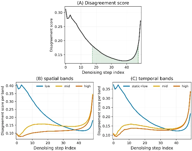
Quantitative evidence. Table 1 reports speedups and VBench temporal metrics over 250 prompts. On Wan 2.1, running the large model for 20 of 50 steps and the small model for the other 30 gives a 1.95× speedup with temporal flicker 96.86 against 96.71 for the all-large model, motion smoothness 98.39 against 98.31, subject consistency 94.81 against 94.62, and background consistency 94.99 against 94.79. On Cosmos 3 the same policy gives 2.04× with the Nano model and 2.73× with the Edge model at 24 of 35 steps; on the four-step TurboDiffusion, 2.69×; on the three-step FastVideo, 2.17×. A human study over 30 prompts with five raters each is reported as comparable in aggregate quality to the all-large baseline. 10
Caveat. The quality result is parity, not improvement, and it rests on VBench's temporal metrics plus a human study of 30 prompts. Calibration is specific to a model pair, so a new large/small pairing needs its own reference rollout before the routing table means anything. All measurements in the paper are recorded on a single NVIDIA A100, and power figures come from NVIDIA's NVML library. 10
Inspectability. No repository, weight release or project page appears in the preprint. The pipelines it modifies — Wan 2.1, Cosmos 3, TurboDiffusion and FastVideo — are public models, but the calibration code and routing tables are not. 10
Why it matters. Serving stacks already keep a distilled small model beside the full one, because that is what step distillation produces. This paper turns that pair into a scheduling decision with an offline calibration run instead of a training job, and it composes with step distillation rather than competing against it: fewer steps, and cheaper steps. The piece to read closely is the disagreement profile, because that shape is what decides how much of a trajectory can be routed away.
2. ViRDM: post-training a video generator without a teacher or a critic
Team and affiliation. Zichong Meng at Northeastern University; Chongjian Ge, Chun-Hao P. Huang and Yang Zhou at Adobe Research; Huaizu Jiang at Northeastern University. The first author's work was done during an internship at Adobe Research, and the two final authors are equal advising. arXiv v1 dated 24 September 2026. 6
What changes. Few-step autoregressive video generators are usually produced by distribution matching distillation, which keeps three video networks alive at once: a frozen teacher to score samples, a learned critic to estimate the distributional discrepancy, and the generator being post-trained. ViRDM asks whether the teacher and the critic can be removed, leaving a generator matched directly against a precomputed target distribution. The recipe comes from one-step image generation, and the paper's real content is the three reasons a direct transfer to video fails. 6
Technical insight. The three barriers and their fixes are the contribution. Backpropagating through a multi-step autoregressive rollout, a VAE decoder and a representation encoder cannot fit in memory at video resolution, so the recipe uses stochastic exits — backpropagating only through the clean-endpoint prediction at one sampled step — together with staged vector–Jacobian products that keep one module's backward graph resident at a time. The image recipe's optimization regime does not carry over: video representation distribution matching saturates at a much smaller fresh population, and cannot turn a bidirectional model into a causal one in twenty updates, so the recipe starts from an existing causal initialization. Representation distributions that describe appearance leave temporal dynamics underconstrained, so a lightweight dynamics regularizer is added. The target distribution is fixed once, from 6,505 real video–text pairs, with V-JEPA 2.1 video features concatenated to normalized SigLIP2 text features. 11
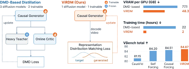
Quantitative evidence. With 20 generator updates, the recipe reaches 84.87 total on the official VBench evaluation against 84.51 for Causal Forcing and 84.20 for Self-Forcing, with quality 85.82 and semantic 81.09. Peak memory per GPU falls from 77.1 GB to 48.3 GB, measured on 81-frame 832×480 videos with one video per GPU, and post-training time from 22 hours to 2 hours on eight A100s; the paper states 16 A100 GPU-hours for the complete recipe. The dynamics regularizer is what closes the motion gap: without it dynamic degree is 48.61 and total 83.41, and with it 72.02 and 84.87. An exploratory extension reports one-, two- and four-step bidirectional generation at 83.12, 84.53 and 84.56 total. 11
Caveat. A user study over 20 prompts puts ViRDM first on text alignment at 40.4%, visual quality at 43.0% and dynamics, but the comparison set is three four-step causal baselines, and the bidirectional extension is labelled exploratory by the authors. The method inherits a requirement rather than creating it: it refines a causal transport that already exists, so the initialization you choose bounds what post-training can reach. The dynamics regularizer is the difference between moderate and strong motion, a gap the authors' own probe shows the video representation cannot resolve on its own. 11
Inspectability. A project page at neu-vi.github.io/ViRDM carries generated videos for each initialization and each configuration, including the ablation that removes dynamics regularization. The preprint announces no code repository and no released weights. 11
Why it matters. Anyone who has paid for a distribution-matching distillation run knows the cost is dominated by keeping a teacher and a critic resident. Removing both changes the shape of the budget: this recipe's 16 A100-hours is a weekend on a small cluster rather than a multi-day job, and the paper's numbers say quality goes up while the cost goes down. The transferable part is the ordering of the three fixes — memory first, initialization second, temporal constraint last — since that is where the image recipe broke.
3. CARE: a representation penalty that reads the conditioning signal
Team and affiliation. Fengjia Guo, Zhuoyi Yang and Jie Tang, all in the Department of Computer Science and Technology at Tsinghua University, Beijing; Guo and Yang are marked equal contribution, with correspondence to Guo and Tang. arXiv v1 dated 23 September 2026. 7
What changes. Representation regularization has become a standard way to speed up diffusion training: align intermediate features, and the model converges sooner. The regularizers in current use apply the same pressure to every sample pair and ignore the conditioning signal — the label or the text — that determines what the model is being asked to generate. CARE starts from the observation that conditions reshape the feature distribution, and that a penalty spread evenly across all pairs spends its strength where it has the least to say. 12
Technical insight. CARE adds a penalty on the representation space whose strength is a function of condition similarity. Pairs whose conditions are close are pushed together hard; pairs whose conditions are far apart are pushed together only weakly. Because the similarity comes from the model's own built-in conditioning signals, the term needs no external alignment loss, no pretrained vision encoder and no extra supervision, and it sits beside the denoising loss as a plug-in. 12
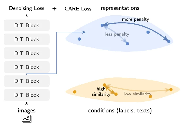
Quantitative evidence. On ImageNet 256×256, SiT-B/2 at 400k steps falls from an FID of 33.02 to 29.71, and SiT-XL/2 at the same point from 17.19 to 13.91, a 19.08% relative improvement; with classifier-free guidance applied, SiT-XL/2 goes from 5.36 to 4.09, a 23.69% relative gain. Training efficiency moves further than quality: the CARE-trained SiT-XL/2 reaches at 2.4M steps an FID below the baseline trained for 7M steps, which is the paper's basis for a 3.5× reduction in training steps. On text-to-image, FID falls from 11.32 to 9.44 at 200k iterations, 16.61%, and from 8.77 to 7.02 at 300k, 19.95%, with the textual CLIP score rising throughout training. Combined with REPA on class-conditioned ImageNet, the best weight on the CARE term moves into the range 0.01 to 0.001. 12
Caveat. Every result is at 256×256 on ImageNet, plus a text-to-image setup the paper reports without a resolution, so the convergence claim is established at the scale the experiments were run rather than at the scale of current image models. The paper also reports that the improvement over a condition-agnostic regularizer narrows when external supervision such as REPA is present, which is a hint about what the term is actually adding. 12
Inspectability. No code, checkpoint or project page appears in the preprint. 12
Why it matters. The practical claim is a training-budget claim, and it is the kind that transfers without the authors' code: if you already use a representation regularizer, the change is to weight each pair by the similarity of its conditions. The measurement to look for in your own runs is the same one the paper reports — the step count at which FID crosses a target — rather than the final FID, because that is where the gain sits.
4. FB-GDM: guidance that calibrates itself
Team and affiliation. Gatien Séguy and Thomas Rodet, SATIE Laboratory, ENS Paris-Saclay, CNRS, Université Paris-Saclay. The preprint is laid out as an IEEE Transactions on Image Processing submission. arXiv v1 dated 24 September 2026. 8
What changes. Two widely used ways to guide a diffusion prior for a linear inverse problem — diffusion posterior sampling, and the pseudoinverse-guided diffusion models the paper abbreviates ΠGDM — both carry scalar hyperparameters that in practice get tuned per task, and usually tuned against the ground truth that the method is supposed to recover. FB-GDM removes that calibration step: the quantities being tuned are inferred from the observation and the forward operator alone. 13
Technical insight. Starting from ΠGDM's Gaussian approximation, the authors derive a closed-form conditional score that depends on two precision parameters — inverse variances, one tied to the denoising approximation and one to the observation likelihood — and treat both as latent variables inferred by variational inference at every reverse step. A separable factorization keeps each update linear in the number of pixels, so full-resolution inference costs about what one ΠGDM run costs. The method's inputs are the observation and the forward operator: no noise level and no ground truth. 13
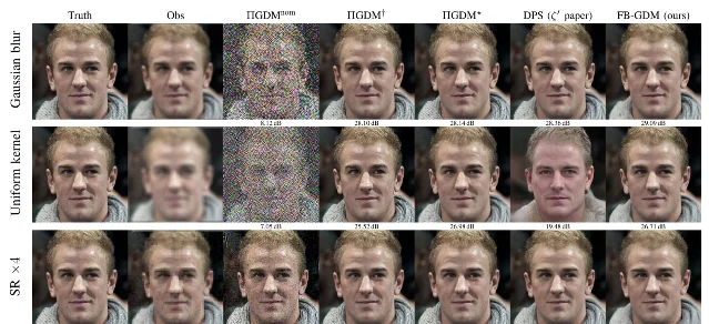
Quantitative evidence. On CelebA-HQ inverse problems the inferred precisions let FB-GDM beat nominal ΠGDM even when ΠGDM is handed the true noise level, by up to 14 dB depending on the operator, and come within 0.1 dB of the ground-truth-calibrated ΠGDM oracle. Figure 3's per-cell PSNR is the readable form: for Gaussian blur, 29.09 dB for FB-GDM against 28.36 dB for diffusion posterior sampling and 28.10 dB for ΠGDM at its nominal setting; for a uniform kernel, 26.71 dB against 19.48 dB for diffusion posterior sampling; for 4× super-resolution, 27.45 dB against 27.27 dB. When the prior is applied to images outside its training set, the paper reports FB-GDM staying faithful where fixed face-prior guidance hallucinates. 13
Caveat. The evaluation is one face dataset with the model's own prior, and the 14 dB figure is the largest gap across operators rather than a typical one; the oracle comparison is against ΠGDM's oracle built on the same Gaussian approximation the method starts from, so it measures how much of that approximation's performance is reachable without calibration. The out-of-distribution test is an illustration of robustness rather than a benchmark. 13
Inspectability. No code link appears in the preprint. The prior it uses is the public
google/ddpm-celebahq-256 checkpoint, so the base model a reader needs is available even though the method is not. 1314Why it matters. Inverse-problem papers are hard to compare because each one's hyperparameters were tuned on the problem it reports. This paper measures the thing that determines whether a method travels: what it does when the operator, the noise level or the image distribution changes, and with no ground truth available to tune against. For anyone applying a diffusion prior to a new measurement operator, the argument to take away is that the data-versus-prior balance can be inferred per step rather than chosen per experiment.
5. AV-GRPO: giving each modality tower its own turn
Team and affiliation. Zhiyu Xu at Shanghai AI Laboratory and The Hong Kong Polytechnic University; Weilong Yan at the National University of Singapore; Yufei Shi at Nanyang Technological University; Shiyang Li at Zhejiang University; Yihao Liu at Shanghai AI Laboratory; Kin-Man Lam at The Hong Kong Polytechnic University and Yuewen Cao at Shanghai AI Laboratory, both marked as corresponding authors. arXiv v1 dated 24 September 2026. 9
What changes. Reinforcement-learning post-training reliably improves a generator that produces one modality, and applying it unchanged to a model that emits audio and video together entangles the two learning signals. A change in the video alters the synchronisation score, so credit cannot be attributed to a modality, and the joint reward can favour different candidates for quality, alignment and synchronisation at once. AV-GRPO converts the coupled problem into a sequence of single-modality ones by making the two towers take turns. 15
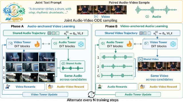
Technical insight. Three pieces do the work. Modality-anchored rollouts freeze one modality as the anchor and sample several candidates of the other against it, which holds the anchor-induced difficulty constant and makes synchronisation rewards comparable across candidates. Trajectory-locked frozen-tower optimization trains one tower per phase while the counterpart stays frozen, which cuts cost and reassigns credit to the tower that actually moved. Adaptive objectives and perturbation strengths then follow each modality's own dynamics. The phases alternate every N training steps: phase A optimizes the video tower against a shared audio trajectory, and phase B optimizes the audio tower against a shared video trajectory. The paper pairs this with 5DAV, a training set decoupled along five dimensions — hierarchy, sound-source type, synchronisation difficulty, temporal complexity and instruction granularity. 15
Quantitative evidence. On JavisBench, full fine-tuning of the 22B LTX-2.3 raises audio quality from 5.097 to 5.798, CLIP from 0.318 to 0.327 and CLAP from 0.408 to 0.468. The cross-modal measures move the most: audio–video ImageBind similarity from 0.212 to 0.247, AVHScore from 0.201 to 0.241, JavisScore from 0.183 to 0.222, and DeSync, where lower is better, from 0.757 to 0.607, with AV-align from 0.354 to 0.398. Against the GDPO baseline the gains sit on the measures where controlling the reference modality matters most: audio–video ImageBind similarity from 0.224 to 0.247, JavisScore from 0.202 to 0.222, and on VABench lip-sync accuracy from 1.439 to 1.646 with DeSync from 0.726 to 0.542. The two training regimes differ in where they win — LoRA takes CLIP 0.330 and DeSync 0.554, both better than the full model's 0.327 and 0.607. 15
Caveat. Two metrics move the wrong way and the paper reports them: LoRA's visual quality is 5.816 against the base model's 5.855, and the fully fine-tuned model's VABench visual-realism score is 4.395 against 4.399 for the base. The evaluation covers one model family and two benchmarks, and the fully fine-tuned result required eight A800 GPUs on a 22B model, so reproducing the headline numbers has a real cost. 15
Inspectability. Code and data are released at zhiyuxu03/AV-GRPO. 16
Why it matters. The synchronisation-reward problem the paper names — a score that depends on which counterpart sample it was computed against — is not specific to audio and video, and the fix is general: hold the other modality fixed and make the comparison fair before you optimize against it. With code and the 5DAV set released, this is also the one paper of the five a reader can run today.
What the five have in common
All five take a number that used to be set once, globally, and make it vary along an axis. TRACK varies model capacity along the denoising trajectory, choosing per step between a large and a small model instead of committing to one for the whole sample. ViRDM varies how many networks stay resident during post-training, from three down to one. CARE varies the strength of the representation penalty pair by pair, according to how similar the two samples' conditions are. FB-GDM varies two precision parameters at every reverse step, per problem, rather than fixing them per task before the run. AV-GRPO varies which tower is being trained, phase by phase. Each paper's method is the rule that sets the varying quantity, and each paper's experiments are the evidence that the rule beats the single global setting it replaced. That is also where to look when deciding whether a result transfers: a rule that reads its value off a quantity you can compute — a disagreement score, a condition similarity, an observation — travels; one that needs the answer in advance does not.
Three of the five sit in
cs.CV and two in cs.LG, and the split falls along the same line as the papers themselves: the three vision entries arrange what is generated and how expensively, and the two machine-learning entries govern the training and inference process behind any generator.A reading order follows from which of those settings is currently open in your own work:
- Start with TRACK if you serve video generation and already keep a distilled small model beside the full one, and want the saving without a retraining run.
- Start with ViRDM if you are budgeting a few-step video post-training run and the teacher–critic stack is what makes it expensive.
- Start with CARE if you are training a diffusion model that already uses a representation regularizer and the training-step count is the constraint.
- Start with FB-GDM if you apply a diffusion prior to a new measurement operator and have no ground truth to tune the guidance against.
- Start with AV-GRPO if you are post-training a joint audio–video model, or if you want to run one of these five yourself this week.
References
- 1arXiv cs.CV new listings
arxiv.org
- 2arXiv cs.LG new listings
arxiv.org
- 3OpenAlex record for arXiv 2609.30096
api.openalex.org
- 4Semantic Scholar record for arXiv 2609.30096
api.semanticscholar.org
- 5TRACK abstract\
arxiv.org
- 6ViRDM abstract\
arxiv.org
- 7CARE abstract\
arxiv.org
- 8FB-GDM abstract\
arxiv.org
- 9AV-GRPO abstract\
arxiv.org
- 10TRACK method
arxiv.org
- 11ViRDM project page
neu-vi.github.io
- 12CARE method
arxiv.org
- 13FB-GDM method
arxiv.org
- 14DDPM CelebA-HQ 256 checkpoint
huggingface.co
- 15AV-GRPO method
arxiv.org
- 16AV-GRPO code and data
github.com
This story was produced automatically by a channel. One sentence is all it takes for Neodrop to keep producing for you.