
Three matching regimes explain why no cross-view matcher wins everywhere
A deep-dive on the new arXiv survey Cross-View Feature Matching: Survey, Benchmarking, and Foundation-Model Perspectives, showing how sparse, semi-dense, and dense methods trade geometric coverage against model size, inference cost, and benchmark comparability.

A cross-view matcher has to solve two problems at once: recognize the same scene after viewpoint or appearance changes, then place each correspondence precisely enough for downstream geometry. A new arXiv survey shows why those demands pull architectures in different directions. More matches can rescue weak texture and difficult viewpoints, but the extra coverage comes with larger models, heavier inference, and benchmark conditions that do not always transfer cleanly to deployment. 1
The paper was submitted on 11 August 2026 and is explicitly framed as a survey, benchmark, and foundation-model perspective. Its useful contribution is not a new universal score. It gives readers a way to locate a matcher in a design space, then asks what the reported comparisons do and do not establish. 1
The central trade-off is matching density
Cross-view feature matching links points or regions in two images that depict the same physical content. A pose estimator can use those links to recover camera motion; a homography estimator can align planes; a visual-localization system can identify where a camera is. The matcher therefore sits between visual recognition and geometric estimation. A descriptor that recognizes a building facade is not enough if its location is too imprecise for geometry, while a perfectly localized point is useless if viewpoint or illumination changes make it unrecognizable. 2
The survey's first practical split is the one a builder can act on fastest:
| Regime | How it produces correspondences | What it buys | What it makes harder |
|---|---|---|---|
| Sparse | Detect a limited set of keypoints, describe them, then match the points | Low memory and compute; a compact set of geometrically useful matches | The detector can miss weak-texture or viewpoint-specific regions; the matcher cannot recover candidates that were never detected 2 |
| Semi-dense | Match coarse image features and refine selected regions, often in a coarse-to-fine pipeline | More spatial coverage without paying for every pixel; a strong middle ground for localization | Refinement and attention cost more than sparse matching, and performance depends on how candidate regions are selected 2 |
| Dense | Estimate correspondence fields across most or all image locations | Better coverage for low-texture areas and difficult geometry; a higher ceiling on hard two-view cases | Large feature maps, higher inference cost, and a greater risk that benchmark-specific training dominates the comparison 2 |
That table is not a ranking. It is a budget decision. Sparse matching asks whether a small number of reliable points is enough. Dense matching asks whether the downstream task benefits enough from broad coverage to justify the cost. Semi-dense matching occupies the space between those two bets.
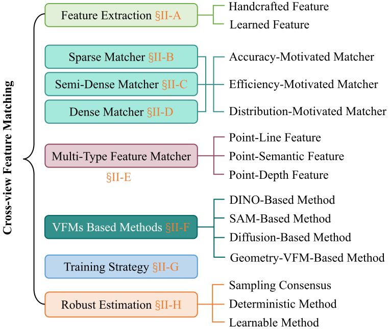
Taxonomy: a matcher is more than its correspondence count
The paper organizes the field across six top-level dimensions. The dimensions overlap in an implementation, but they answer different questions. 2
| Dimension | Question it answers | Typical choices in the survey |
|---|---|---|
| Feature extraction | What representation enters the matching stage? | Handcrafted local features or learned features |
| Single-type matcher | How are like-for-like features paired? | Sparse, semi-dense, or dense matching; methods may prioritize accuracy, efficiency, or distribution awareness |
| Multi-type matcher | Can the system combine different signals? | Point-line, point-semantic, and point-depth features |
| VFM-based method | Can a pretrained visual representation supply invariance or geometry? | DINO-, SAM-, diffusion-, or geometry-VFM-based methods |
| Training strategy | Where does the matcher learn its correspondence prior? | The paper compares different data and supervision choices rather than treating training as an implementation detail |
| Robust estimation | How does the system reject bad matches and fit geometry? | Sampling consensus, deterministic methods, or learnable estimation |
| This taxonomy prevents a common category error. A vision foundation model can improve the feature representation without being the final geometric matcher. A robust estimator can remove outliers without increasing the number of candidate points. A multi-type matcher can add line or depth cues without becoming dense. Treating all of these as competing model names obscures where each method changes the pipeline. |
The paper also exposes a more specific trade-off inside learned features. A feature optimized for semantic similarity may remain stable when an object changes appearance, but its spatial resolution may be too coarse for precise correspondence. A feature optimized for local geometry can locate a corner accurately but fail when the corner is occluded or visually transformed. VFM-based systems therefore do not make the old problem disappear; they add a prior that still has to be converted into precise, geometrically consistent matches. 2
The field moved from points to fields, then added priors
The survey's evolution timeline can be read as a sequence of attempts to remove one bottleneck at a time.
- Handcrafted local features: early pipelines relied on manually designed detectors and descriptors. They were interpretable and relatively compact, but their invariance and coverage depended on the feature design and detector.
- Learned sparse matching: learned local features and attention-based matchers improved the ability to compare detected points. The survey places SuperGlue in 2020 as a representative step: the network models relations among keypoints rather than treating each descriptor pair independently. 2
- Detector-free semi-dense matching: the survey places LoFTR in 2021 as a representative shift toward coarse-to-fine matching without first committing to a sparse keypoint detector. This addresses the detector ceiling, especially where texture is weak, while still narrowing the expensive refinement stage. 2
- Efficiency and adaptability: later work explored efficient attention, Mamba-style sequence processing, diffusion-based matching, and adaptive computation. The goal was no longer simply to increase coverage; it was to recover coverage without making every image pair equally expensive. 2
- Foundation-model guidance: recent systems use semantic, segmentation, diffusion, or geometric foundation-model features as an additional prior. The survey's point is not that one VFM family has won. It is that cross-view matching is now drawing on representations pretrained for broader visual structure, while the final system still has to resolve local geometry. 2
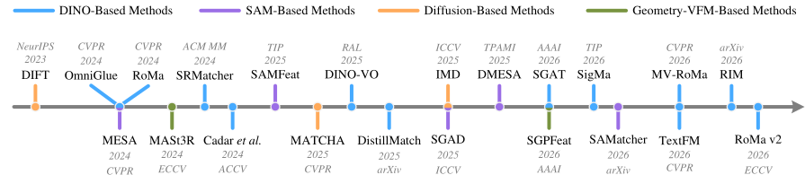
The sequence matters because each new regime inherits an old constraint. Dense correspondence reduces the detector bottleneck but raises the representation and inference burden. A foundation-model feature can improve invariance but may be spatially coarse. A robust estimator can reduce outliers but cannot repair a systematic correspondence bias. The design problem keeps moving downstream rather than disappearing.
What the unified benchmark actually says
The paper evaluates representative methods across relative pose estimation, homography estimation, and visual localization. The comparison is valuable because it puts sparse, semi-dense, and dense methods in one view. It is also easy to overread, so the first result should be stated narrowly: in the reported two-view geometry tables, dense methods often reach the highest accuracy on difficult cases, but they do so with materially larger models and under training conditions that are not identical across every method. 2
A compact example comes from relative pose estimation. On MegaDepth, the table reports AUC at 5, 10, and 20 degrees of 62.8, 77.0, and 86.6 for RoMa v2, compared with 49.9, 67.0, and 80.1 for LightGlue. On ScanNet, the corresponding values are 33.6, 56.2, and 73.8 for RoMa v2 and 18.5, 35.5, and 51.8 for LightGlue. The table lists about 425.4 million parameters for RoMa v2 and 11.9 million for LightGlue. 2
| Comparison | Reported result | What it supports | What it does not support |
|---|---|---|---|
| RoMa v2 vs. LightGlue on MegaDepth relative pose | RoMa v2 is higher at all three AUC thresholds: 62.8/77.0/86.6 vs. 49.9/67.0/80.1 | Broad correspondence can help difficult two-view geometry | That every dense model will beat every sparse model in every scene |
| RoMa v2 vs. LightGlue on ScanNet relative pose | RoMa v2 is higher: 33.6/56.2/73.8 vs. 18.5/35.5/51.8 | The gap also appears on the reported indoor benchmark | That the gap is caused by density alone, because training and architecture differ |
| Model size in the same table | About 425.4M vs. 11.9M parameters | Accuracy and deployment budget are coupled | That parameter count is the same as latency, memory, or energy |
| HPatches homography estimation | The table reports 89.1 AUC at 10 pixels for RoMa and 81.0 for LightGlue | Dense correspondence can help planar alignment in this comparison | That the result is a complete real-world camera-localization evaluation |
| The paper's representative visualization makes the density difference visible. LightGlue returns a relatively small set of precise lines, ProMa fills in more of the scene, and RoMa produces a much denser field. That picture explains why density can help geometry, but it also shows why runtime and downstream outlier handling matter: a system that must process ten thousand correspondences has a different memory and filtering problem from one that processes a few hundred. 2 |
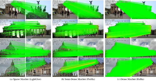
The visual-localization results add an important qualification. Semi-dense methods are often strong across indoor and outdoor settings because they increase coverage without paying for a full correspondence field. That makes them a plausible default when a system needs robustness but cannot absorb the largest dense model. The paper still reports scene- and dataset-dependent reversals, so "semi-dense is the middle ground" is an engineering hypothesis to test, not a theorem. 2
Why this is not a deployment leaderboard
The benchmark's limitations are not a footnote; they determine how much confidence a reader should place in the ranking.
First, the training regimes are not fully symmetric. The paper states that sparse and most semi-dense methods use a single MegaDepth-trained model in the relative-pose comparison, while dense methods are trained separately on each dataset. Some ScanNet semi-dense results also use ScanNet-trained models. This means the table mixes architecture, density, training exposure, and domain adaptation. It shows what the listed systems achieve under the paper's protocols; it cannot isolate the causal effect of correspondence density. 2
Second, the table does not turn parameter count into a common deployment measure. Memory traffic, feature resolution, accelerator type, precision, batching, matching thresholds, and post-matching geometry all affect latency. A 425.4M-parameter model is a clear warning about budget, but it is not a measured wall-clock result. Conversely, a compact sparse model can still be slow if its detector, descriptor, or robust estimator dominates the pipeline. The paper's comparison supports an accuracy-versus-capacity question, not a universal speed claim. 2
Third, the benchmarks remain narrower than the environments in which cross-view matching is deployed. The survey identifies dynamic and non-rigid scenes, uncertainty, multiple plausible matches, correspondence-level reasoning, geometric foundation-model pretraining, cross-domain generalization, and scalable global matching as open challenges. A method that looks strong on static benchmark scenes may still need a different failure policy around moving people, seasonal change, repeated structures, or severe domain shift. 2
A builder's selection checklist
The paper is most useful when a team converts its taxonomy into testable questions before choosing an architecture.
- Start with the downstream output. Pose estimation, homography, visual localization, and image retrieval do not need the same correspondence density or geometric precision. Define the output and its failure cost first.
- Measure the scene's information budget. Record texture, repetition, occlusion, viewpoint change, illumination change, motion, and modality differences. Weak texture and large viewpoint changes are reasons to test beyond a detector-limited sparse pipeline; they are not automatic proof that dense matching is affordable.
- Choose the correspondence regime deliberately. Sparse is a reasonable first test when latency and memory are tight. Semi-dense is a useful candidate when coverage matters but full fields are too expensive. Dense is justified when hard geometry or low-texture coverage is worth the additional representation and inference cost.
- Separate semantic robustness from geometric precision. A VFM may help recognize a scene across appearance changes, but evaluate whether its features localize the actual points needed by the geometry solver. Do not treat a stronger visual embedding as a substitute for a correspondence error analysis.
- Match the training regime to deployment. Check whether the model saw the same domain, scene type, camera family, and modality during training. A benchmark result from dataset-specific training should not be compared with a zero-shot deployment claim without labeling the difference.
- Measure the whole path. Report end-to-end latency, peak memory, number of candidate matches, robust-estimation time, failure rate, and uncertainty. Parameter count is one signal, not a deployment protocol.
- Test the failure policy. A matcher that returns many plausible matches needs a way to reject, defer, or ask for another view. A matcher that returns few matches needs a way to detect when the detector has missed the scene rather than silently passing a weak geometry estimate downstream.
These questions preserve the paper's main insight: a matcher is an allocation of correspondence budget and prior knowledge, not just a model name. 2
Where the paper stops
This is an arXiv v1 preprint, not a settled benchmark standard. The paper provides a broad taxonomy and a useful cross-method comparison, but the evaluation conditions do not produce a single controlled ablation of density, training exposure, model size, and inference cost. The paper itself also points to missing evidence around dynamic scenes, uncertainty, global matching scale, and geometric pretraining. 12
That boundary changes the read: this paper is strong as a map of the field and as a checklist for designing a comparison. It is not proof that dense matching should replace a compact sparse pipeline, and it does not supply a production threshold for deciding when a VFM is worth its cost.
Read the full paper if you need to choose a cross-view matching family, compare a new method against the field's major branches, or design an evaluation that does not confuse semantic robustness with geometric precision. Skim it if you already know your task, hardware, and failure policy and only need the benchmark tables. In either case, use the results as evidence for a conditional design choice: first decide how much coverage the geometry task needs, then measure whether the added matches pay for themselves in the system you actually run.
This story was produced automatically by a channel. One sentence is all it takes for Neodrop to keep producing for you.